In [3] we have introduced a controllability principle for a general control problem related to operator equations. It consists in finding $(w,\lambda ),$ a solution to the following system

involving the fixed point equation $w=N(w,\lambda ).$ Here $w$ is the state variable, $\lambda$ is the control variable, $W$ is the domain of the states, $\mathrm{\Lambda }$ is the domain of controls and $D\subset W\times \mathrm{\Lambda }$ is the controllability domain given expression to a certain condition/property imposed to $w,$ or to both $w$ and $\lambda .$ There are no structure imposed to the sets $W,\mathrm{\Lambda }$ and $D$ and no properties for the mapping $N$ from $W\times \mathrm{\Lambda }$ to $W.$

We say that the equation $w=N(w,\lambda )$ is controllable in $W\times \mathrm{\Lambda }$ with respect to $D,$ if problem (1.1) has a solution $(w,\lambda )$. In case that the solution is unique, we say that the equation is uniquely controllable.

In order to describe the solving of the general control problem, let us define the sets

Obviously, the solutions of the control problem (1.1) are the elements of $\mathrm{\Sigma }\cap D.$

Consider now the set-valued map $F:{\mathrm{\Sigma }}_1\to \mathrm{\Lambda }$  given by

Notice that $F$ gives us the expression of the control variable according to the state variable.

The next propositions is a general principle for solving the control problem (1.1).

In many applications $F$ and $\tilde{F}$ are single-valued maps and $F$ can be extended to $W$ by simply using its very expression.

Two applications for a system modeling cell dynamics related to leukemia have been included in [3] (see also [5]) and three others in [6], from which two self-control problems. Many other illustrations of the above principle can be derived from the rich literature in control theory (see, e.g., the monograph [2]).

The aim of this note is to give an algorithm for approximation of the solutions of general control problems. It basically  consists of a bisection method for the control variable inside an interval associated to a pair of lower and upper solutions. The notions of lower and upper solutions for a general control problem are defined accordingly.

First, we introduce in the present set-framework the notions of lower and upper solutions of a control problem. To this aim, we assume a certain partition of the solution domain

which allows us to say that the condition of controllability is targeted from the left or from the right. Thus, we can give the following definition.

In contrast to the statement of the controllability principle from above, given in unstructured  sets, from now on we shall assume a certain topological structure of the sets and accordingly the continuity of the map $N.$ The topological framework is a natural one for approximation methods, when a certain meaning is required for the terms of approximant and of method convergence.

Assume that $W$ is a metric space, $\mathrm{\Lambda }=conv\{{\underset{¯}{\lambda }}_0,{\overline{\lambda }}_0\}$ is a segment of a normed space with norm $\parallel \cdot \parallel ,$ and that the sets $\underset{¯}{D},\overline{D}$ are closed.

In addition, assume that the following conditions are satisfied:

(h1)

The problem admits a lower solution of the form $({\underset{¯}{w}}_0,{\underset{¯}{\lambda }}_0)$ and an upper solution $({\overline{w}}_0,{\overline{\lambda }}_0);$

(h2)

For each $\sigma \in [0,1],$ there exists a unique $w=:S\left(\sigma \right)\in W$ with $(w,\lambda )\in \mathrm{\Sigma }$ for $\lambda =\lambda \left(\sigma \right):=\left(1-\sigma \right){\underset{¯}{\lambda }}_0+\sigma {\overline{\lambda }}_0;$

(h3)

The map $S:$ $[0,1]\to W$ is continuous.

We use now the following bisection algorithm.

The algorithm leads either to a solution when it stops, or to two sequences $\left({\underset{¯}{\sigma }}_k\right)$ and $\left({\overline{\sigma }}_k\right)$ such that

(i)

$0\le {\underset{¯}{\sigma }}_1\le \mathrm{\cdots }\le {\underset{¯}{\sigma }}_k\le {\underset{¯}{\sigma }}_{k+1}\le \mathrm{\cdots }\le 1$and$(S\left({\underset{¯}{\sigma }}_k\right),\lambda \left({\underset{¯}{\sigma }}_k\right))\in \underset{¯}{D},$

(ii)

$0\le \mathrm{\cdots }\le {\overline{\sigma }}_{k+1}\le {\overline{\sigma }}_k\le \mathrm{\cdots }\le {\overline{\sigma }}_1\le 1$and$(S\left({\overline{\sigma }}_k\right),\lambda \left({\overline{\sigma }}_k\right))\in \overline{D},$

(iii)

$0\le {\overline{\sigma }}_k-{\underset{¯}{\sigma }}_k=\frac{1}{2^k}.$

Then the sequences $\left({\underset{¯}{\sigma }}_k\right)$ and $\left({\overline{\sigma }}_k\right)$ are convergent and in virtue of (iii) their limits are equal, say ${\sigma }^{\ast }.$ Clearly, ${\sigma }^{\ast }\in [0,1].$ Furthermore, using the continuity of $S$ and the fact that $\underset{¯}{D},\overline{D}$ are closed, from $(S\left({\underset{¯}{\sigma }}_k\right),\lambda \left({\underset{¯}{\sigma }}_k\right))\in \underset{¯}{D}$ we obtain $(S\left({\sigma }^{\ast }\right),\lambda \left({\sigma }^{\ast }\right))\in \underset{¯}{D}.$ Similarly $(S\left({\sigma }^{\ast }\right),\lambda \left({\sigma }^{\ast }\right))\in \overline{D}.$ Hence $(S\left({\sigma }^{\ast }\right),\lambda \left({\sigma }^{\ast }\right))\in D$ that is $(S\left({\sigma }^{\ast }\right),\lambda \left({\sigma }^{\ast }\right))$ solves the control problem and proves the convergence of the algorithm. Thus, we have proved the following theorem.

An example. Consider the Lotka-Volterra model with seasonal harvesting

where $g,h\in L^1(0,T).$

Assume that for two routine harvesting policies $(g_1,h_1)$ and $(g_2,h_2),$ the ratio between the two species $x\left(T\right)/y\left(T\right)$ at the end $T$ of a season is below and respectively, above a desired level $r.$ The control problem is to find the appropriate harvesting policy $(g,h)$ to achieve the ratio $r$ considered optimal. Clearly, under some given initial values $x_0,y_0,$ the system (2.1) reads equivalently as a fixed point equation

Compared to the abstract control problem stated in Section 1, here $w=(x,y),\lambda =(g,h),$ $W=C([0,T];{(0,+\mathrm{\infty })}^2),$ ${\underset{¯}{\lambda }}_0=(g_1,h_1),$ ${\overline{\lambda }}_0=(g_2,h_2),$ $\mathrm{\Lambda }=\{(g_{\sigma },h_{\sigma }):\sigma \in [0,1]\},$ where $g_{\sigma }=\left(1-\sigma \right)g_1+\sigma g_2,$ $h_{\sigma }=\left(1-\sigma \right)h_1+\sigma h_2,$

Also, according to Definition 2, $(x_1,y_1,g_1,h_1)$ and $(x_2,y_2,g_2,h_2)$ (with $(x_i,y_i)$ the solution of system (2.2) for $g=g_i$ and $h=h_i,i=1,2$) are lower and upper solutions of the control problem, respectively.

Notice that it seems natural that the appropriate policy should be an intermediary between the two routine policies. Our algorithm looks for it as a convex combination of the two routine strategies and thus the control problem reduces to finding $\sigma \in [0,1]$ for which the solution $(x,y)$ of the system

with $g_{\sigma }=\left(1-\sigma \right)g_1+\sigma g_2,$ $h_{\sigma }=\left(1-\sigma \right)h_1+\sigma h_2$ and some given initial values $x_0,y_0,$ satisfy

In the paper [10] (see also [7]) the following system has been introduced as a model of cell dynamics after bone marrow transplantation

Here $x\left(t\right),y\left(t\right),z\left(t\right)$ stand for the normal, leukemic and donor cell populations at time $t,$ after transplant time $t=0$ when their concentrations are supposed to have been $x_0,y_0,z_0\left(>0\right).$ Parameters $a,A$ stand for the growth rates of normal and leukemic cells; $c,C$ are their cell death rates; and $b,B$ are their microenvironment sensitivity rates. Also, the parameters $h,g,G$ stand for the intensity of anti-graft, anti-host and anti-leukemia effects, respectively.  They totalize a large number of cell biophysical properties, as well as exterior stimulants and inhibition during the immunotherapy. Values of the parameters $h,g,G$ close to zero correspond to weak interactions, larger values quantify strong effects and their pre-transplant estimate would be crucial for transplant strategy (conditioning treatment, dose of infused cells and post-transplant immunosuppressive therapy). We note that the model was refined in [4] by considering instead of the same sensitivity rate $b$ for normal and leukemic cells, different sensitivity rates $b_1$ and $b_2$, respectively.

In paper [8], the equilibria of system (3.1) are found and their stability is established in terms of the system parameters. According to the main result in [8] the system has, as the numerical simulations in [9] suggested, only two asymptotically stable equilibria, namely the ”bad” equilibrium $P_2(0,D,0)$ and the ”good” one $P_3(0,0,d).$ Here the values

can be seen as homeostatic normal and cancer levels. Also, the octant of the positive states $(x,y,z)$ splits into two basins of attraction of the two equilibria, the ”bad” basin corresponding to $(0,D,0),$ and the ”good” one for $(0,0,d)$ (see Fig. 1 and the Appendix for its construction). This means that if at a given time $t_0$ the state $(x\left(t_0\right),y\left(t_0\right),z\left(t_0\right))$ belongs to the basin of attraction of any of the two equilibria, then the entire trajectory $(x\left(t\right),y\left(t\right),z\left(t\right))$ for $t\ge t_0$ remains in the same basin and, as a result, in time, approaches the corresponding equilibrium. Thus, a transplant appears as successful if the initial state $(x_0,y_0,z_0)$ is located in the good basin, which happens if $z_0$ is sufficiently large compared with $x_0$ and $y_0.$ Also, an unsuccessful transplant could be turned into a successful one if by any methods/therapies one can move the state $(x,y,z)$ from the bad basin into the good one, or if we can enlarge the good basin to catch the state inside. In fact, for any transplant, one could preventively apply the same strategy in order to move the state $(x,y,z)$ (even if located in the good basin) away from the separating surface between the two basins, to be sure that further perturbations can not change the good evolution towards equilibrium $(0,0,d).$

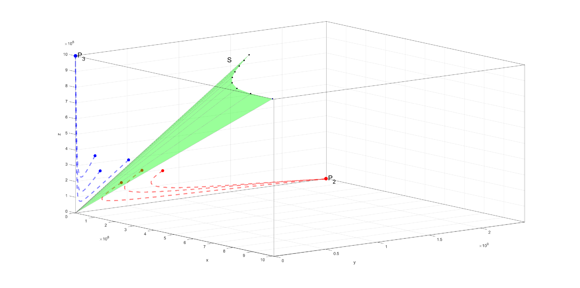
From the main result in [8] we have that the separation surface $S$ of the two basins of attraction intersects the plane $y=0$ after the line

and the plane $x=0$ after a curve closed to the line

Thus, the good basin of attraction increases if at least one of the two lines goes down, which happens if one can make $h/g$ or/and $A/C$ to decrease, or/and $G$ to increase.

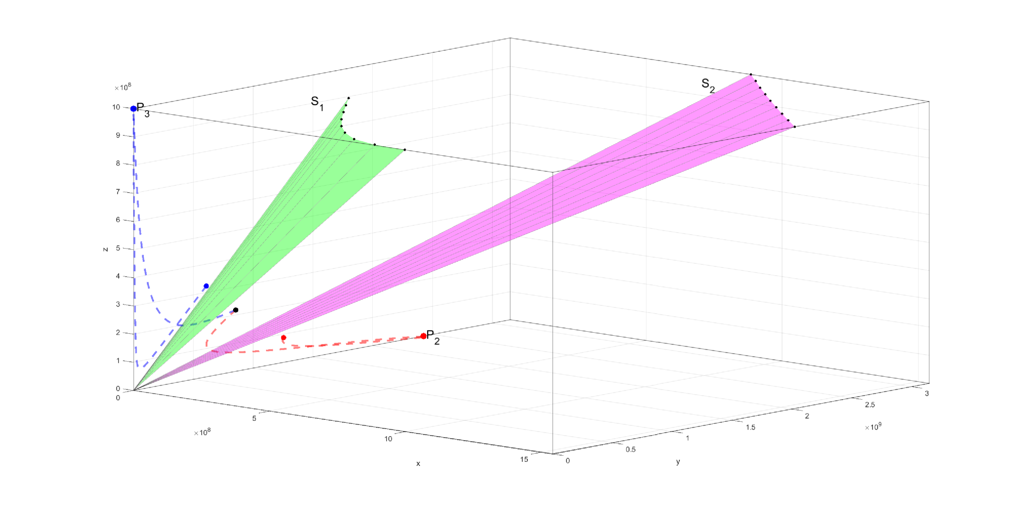
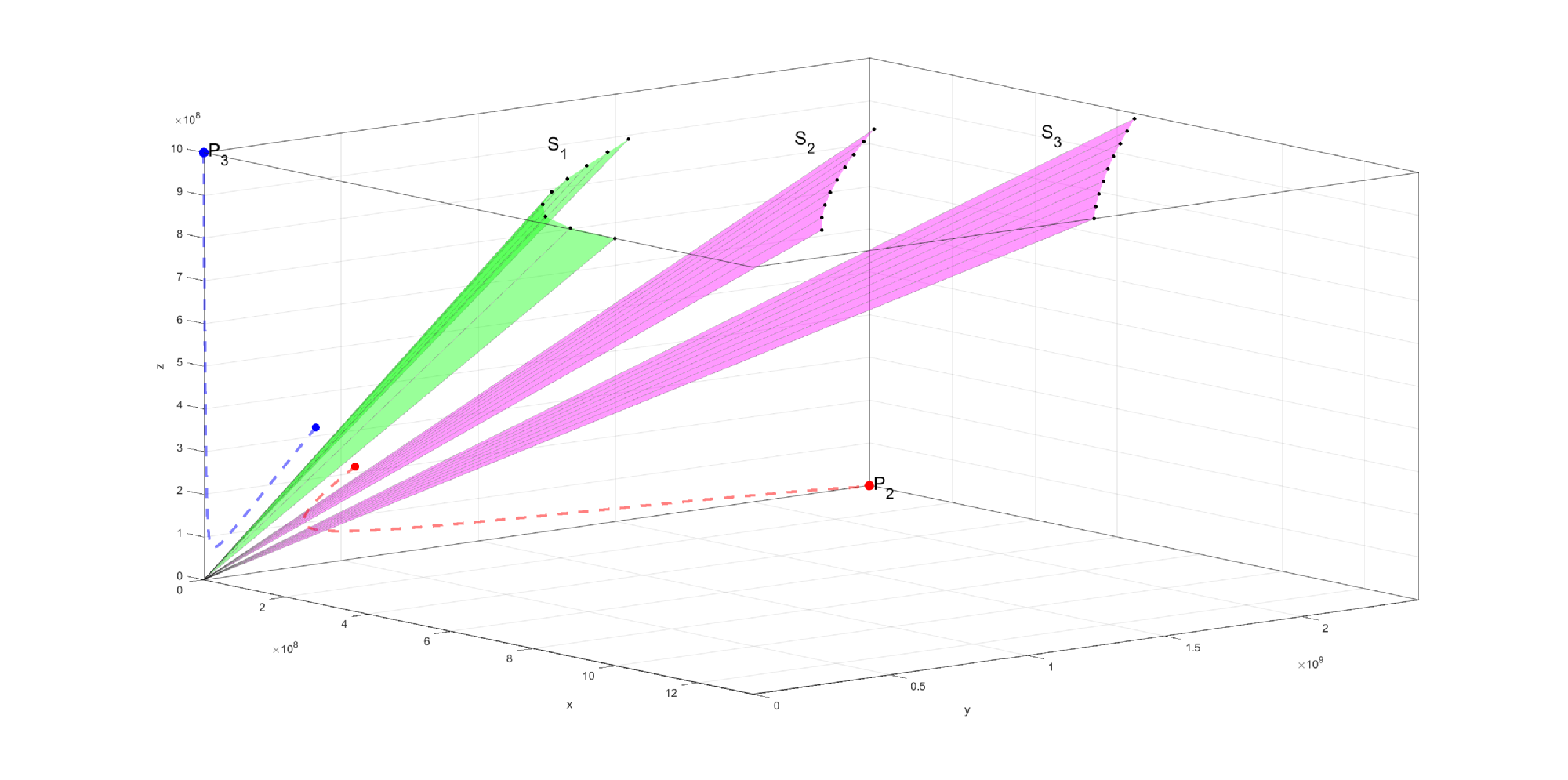
Therefore, the basin of attraction of the good equilibrium $P_3$ is enlarged if the separation surface $S$ goes down (see Fig. 2 and Fig. 3) and this can be achieved by

1. 1.

   decreasing of anti-graft parameter $h;$

2. 2.

   increasing of anti-host parameter $g;$

3. 3.

   increasing of anti-cancer parameter $G;$

4. 4.

   decreasing of growth rate of cancer cells $A;$

5. 5.

   increasing of death rate of cancer cells $C.$

Such changes in these parameters find their counterpart in post-transplant medical practice, namely the following therapies: immunosuppressive therapy (related to $h$), post-transplant consolidation chemotherapy (related to $A$ and $C$) and donor T-lymphocyte infusion (related to $g$ and $G$). In [9] a series of imaginary scenarios combining these therapies have been designed and it has been shown that success depends on their intensity, the time interval in which they are applied and the time after transplantation at which they are initiated.

Denote by ${\lambda }_i\left(t\right),i=1,2,\mathrm{\dots },5$ the factors with which the parameters $h,g,G,A$ and $C$ are modified on a time interval $[0,T]$ and assume that as functions they belong to $L^{\mathrm{\infty }}(0,T).$ For example, we can consider these functions piecewise constant, when the value one on a certain subinterval would correspond to an interruption of the therapy. Also, denote by $\lambda \left(t\right)$ the vector in ${ℝ}^5$ having these components.

Assuming that after transplant one has $y\simeq 0$ on the time interval $[0,T]$ and that the patient’s condition $w_0=(x_0,y_0,z_0)$ is in the bad basin, that is, we want to decrease the $h/g$ ratio to reach the goal

meaning that the patient’s condition is brought to time $T$ in the good basin, evolving after that to the good attractor $P_3$. Obviously, the patient’s exposure to corrective therapies should be reduced as much as possible. In order to find such a minimal therapy according to $\lambda \left(t\right)$ we can apply our lower and upper solution method.

Clearly, for a lower solution $({\underset{¯}{x}}_0,{\underset{¯}{y}}_0,{\underset{¯}{z}}_0,{\underset{¯}{\lambda }}_0)$we can take the vector ${\underset{¯}{\lambda }}_0=(1,1,1,1,1)$ which corresponds to the absence of any post-transplant therapy. Then

An upper solution $({\overline{x}}_0,{\overline{y}}_0,{\overline{z}}_0,{\overline{\lambda }}_0)$can be chosen by checking several vector functions $\lambda \left(t\right)$ with step function components satisfying $0\le {\lambda }_i\left(t\right)\le 1$ for $i=1,4$ and ${\lambda }_i\left(t\right)\ge 1$ for $i=2,3,5.$ For it one has

Once this upper solution is found, the algorithm starts and continues until the first step $k$ at which, for $\lambda =\lambda \left({\overline{\sigma }}_k\right),$ one has

for an acceptable margin Then the vector $\lambda \left({\overline{\sigma }}_k\right)=\left(1-{\overline{\sigma }}_k\right){\underset{¯}{\lambda }}_0+{\overline{\sigma }}_k{\overline{\lambda }}_0$ can be a good approximation for the control $\lambda .$

In this case, referring to the general framework, we have $W=C([0,T];{(0,+\mathrm{\infty })}^3),w=(x,y,z),$ $\mathrm{\Lambda }=\{\lambda \left(\sigma \right):\sigma \in [0,1]\},$ where $\lambda \left(\sigma \right)=\left(1-\sigma \right){\underset{¯}{\lambda }}_0+\sigma {\overline{\lambda }}_0,$

Also $N=(N_1,N_2,N_3)$ is the integral operator associated to the equivalent integral system.

First, we prove that the solution operator $S$ is well-defined, that is condition (h2) holds.

Finally, we prove the continuous dependence on $\sigma$ of the solution $S\left(\sigma \right)=(x,y,z),$ that is condition (h3).

LG Parajdi benefited from financial support through the project ”Development of advanced and applied research skills in the logic of STEAM+ Health”, POCU/993/6/13/153310, a project co-financed by the European Social Fund through the Human Capital Operational Program 2014-2020.

We aim to build numerically the surface $S$ that separates the basin of attraction of the ”good” attractor (when the bone marrow transplant succeeds) from the basin of the ”bad” attractor (when the transplant fails). Let $C$ be the curve at the intersection between the surface $S$ and the horizontal plane at $z=\tilde{z}$. For numerical tractability, we approximate the surface $S$ by a ruled surface which connects the origin of the axes with the curve $C$.

The surface $S$ intersects the plane $x=0$ approximately along a line

and the plane $y=0$ along the line

The above two lines intersect the plane $z=\tilde{z}$ in the points

respectively. We wish to compute the coordinates of $N-1$ points on the curve $C$. To this end,

1. Let there be an equidistant partition of the segment $M_0{M}_1$, i.e. a series of points

where

and

such as the points $M_{k/N}$ divide the segment $M_0{M}_1$ into $N$ equal parts. Equivalently, in vector notation:

Componentwise, we have

2. For each $k=1,2,\mathrm{\dots },N-1$ we compute the following: Let there be in the plane $z=\tilde{z}$ the normal on $M_0{M}_1$ in $M_{k/N}$ and, on this normal, two series of equidistant points ${\underset{¯}{S}}_i,{\overline{S}}_i$, spaced at $\epsilon$ from each other

that is the points are situated on the normal on $M_0{M}_1,$ on opposite sides of $M_{k/N}.$ Vectorially

where $\overrightarrow{v}$ is the unit vector orthogonal to $\overrightarrow{M_1{M}_0},$ that is

Componentwise, for all points ${\underset{¯}{S}}_i,{\overline{S}}_i$ we have

and respectively

To find an approximation of the surface $S$ we have employed the following pseudocode algorithm (implemented in Matlab R2021a):

FOR each $k=1,2,\mathrm{\dots },N-1$ we test whether the point $M_{k/N}$ lies inside the good or the bad basin of attraction, by following the trajectory of the solution that starts from that point (integrating using the coordinates of the point $M_{k/N}$ as initial conditions).

IF the trajectory leads to the bad attractor, we test in sequence the orbits of the points ${\underset{¯}{S}}_i$, $i=1,2,\mathrm{\dots }$, until we reach the first point whose orbit lands on the good attractor. The midpoint of the segment determined by the last two tested points will belong, within an $\epsilon /2$ approximation, to the curve $C$ / surface $S$.

IF the trajectory leads to the good attractor, we test in sequence the orbits of the points ${\overline{S}}_i$, $i=1,2,\mathrm{\dots }$, until we reach the first point whose orbit lands on the bad attractor. The midpoint of the segment determined by the last two tested points will belong, within an $\epsilon /2$ approximation, to the curve $C$ / surface $S$.

END_FOR

Every point on the curve $C$, as found above, is then connected with the origin. The resulting ruled surface is a rough but useful approximation of the surface $S$, computable in linear time with respect to $N$ and $1/\epsilon$.

Concerning the parameters for these simulations (see Fig. 1, Fig. 2 and Fig. 3), the following values are taken: $a=0.23,b=2.2\times {10}^{-8},c=0.01,A=0.43,B=5.5\times {10}^{-9},C=0.03,g=25,G=4,h=20,$ where . In all the simulations we have used the following values for $N=10$, $\epsilon ={10}^8$, $\tilde{z}={10}^9$.

References

- [1] Barbu, V.: Differential Equations, Springer, Cham (2016). https://doi.org/10.1007/978-3-319-45261-6
- [2] Coron, J.-M.: Control and Nonlinearity, Mathematical Surveys and Monographs Vol. 136, Amer. Math. Soc., Providence (2007). https://doi.org/http://dx.doi.org/10.1090/surv/136
- [3] Haplea, I.Ş., Parajdi, L.G., Precup, R.: On the controllability of a system modeling cell dynamics related to leukemia, Symmetry 13(10), 1867 (2021). https://doi.org/10.3390/sym13101867
- [4] Parajdi, L.G.: Stability of the equilibria of a dynamic system modeling stem cell transplantation, Ric. Mat. 69(2), 579–601 (2020). https://doi.org/10.1007/s11587-019-00473-9
- [5] Parajdi, L.G., Patrulescu, F.O., Precup, R., Haplea, I.Ş.: Two numerical methods for solving a nonlinear system of integral equations of mixed Volterra-Fredholm type arising from a control problem related to leukemia, submitted.
- [6] Precup, R.: On some applications of the controllability principle for fixed point equations, Results Appl. Math. 13, 100236 (2022). https://doi.org/10.1016/j.rinam.2021.100236
- [7] Precup, R., Dima, D., Tomuleasa, C., Şerban, M.-A., Parajdi, L.-G.: Theoretical Models of Hematopoietic Cell Dynamics Related to Bone Marrow Transplantation, in Frontiers in Stem Cell and Regenerative Medicine Research. Volume 8, eds Atta-ur-Rahman, Shazia Anjum, Bentham Science, Sharjah, pp 202–241 (2018). https://doi.org/10.2174/9781681085890118080008
- [8] Precup, R., Şerban, M.-A., Trif, D.: Asymptotic stability for a model of cell dynamics after allogeneic bone marrow transplantation, Nonlinear Dyn. Syst. Theory 13(1), 79–92 (2013). https://www.e-ndst.kiev.ua/v13n1/7(42).pdf
- [9] Precup, R., Şerban, M.-A., Trif, D., Cucuianu, A.: A planning algorithm for correction therapies after allogeneic stem cell transplantation, J. Math. Model. Algor. 11(3), 309-323 (2012). https://doi.org/10.1007/s10852-012-9187-3
- [10] Precup, R., Trif, D., Şerban M.-A., Cucuianu, A.: A mathematical approach to cell dynamics before and after allogeneic bone marrow transplantation, Ann. Tiberiu Popoviciu Semin. Funct. Equ. Approx. Convexity 8, 167–175 (2010). http://atps.tucn.ro/pdf/8-2010-atps-abstracts.pdf
Appendix: A numerical method for constructing the separation
surface between the two basins of attraction
We aim to build numerically the surface that separates the basin of
attraction of the ”good” attractor (when the bone marrow transplant
succeeds) from the basin of the ”bad” attractor (when the transplant fails).
Let be the curve at the intersection between the surface and the
horizontal plane at . For numerical tractability, we
approximate the surface by a ruled surface which connects the origin of
the axes with the curve .
The surface intersects the plane approximately along a line
and the plane along the line
The above two lines intersect the plane in the points