Abstract
This work is about the use of some classical spectral collocation methods as well as with the new software system Chebfun in order to compute the eigenpairs of some high order Sturm–Liouville eigenproblems. The analysis is divided into two distinct directions. For problems with clamped boundary conditions, we use the preconditioning of the spectral collocation differentiation matrices and for hinged end boundary conditions the equation is transformed into a second order system and then the conventional ChC is applied. A challenging set of “hard” benchmark problems, for which usual numerical methods (FD, FE, shooting, etc.) encounter difficulties or even fail, are analyzed in order to evaluate the qualities and drawbacks of spectral methods. In order to separate ‘‘good” and “bad” (spurious) eigenvalues, we estimate the drift of the set of eigenvalues of interest with respect to the order of approximation N. This drift gives us a very precise indication of the accuracy with which the eigenvalues are computed, i.e., an automatic estimation and error control of the eigenvalue error. Two MATLAB codes models for spectral collocation (ChC and SiC) and another for Chebfun are provided. They outperform the old codes used so far and can be easily modified to solve other problems.
Authors
Calin-Ioan Gheorghiu
“Tiberiu Popoviciu” Institute of Numerical Analysis, Romanian Academy
Keywords
Sturm–Liouville; clamped; hinged boundary condition; spectral collocation; Chebfun; chebop; eigenpairs; preconditioning; drift; error control
References
see the expanding block below
Cite this paper as:
C.I. Gheorghiu, Accurate spectral collocation solutions to 2nd-order Sturm–Liouville problems, Symmetry, 13 (2021) 3, 385, doi: 10.3390/sym13030385
About this paper
Print ISSN
Not available yet.
Online ISSN
2073-8994
Google Scholar Profile
soon
Paper (preprint) in HTML form
Accurate Spectral Collocation Solutions to 2nth-Order Sturm-Liouville Problems.
Abstract
This work is about the use of some classical spectral collocation methods as well as about the use of the new software system Chebfun in order to compute the eigenpairs of some high order Sturm-Liouville eigenproblems. The analysis is divided into two distinct directions. For problems with clamped boundary conditions we use the preconditioning of the spectral collocation differentiation matrices and for hinged end boundary conditions the equation is transformed into a second order system and then the conventional ChC is applied. A challenging set of “hard”benchmark problems, for which usual numerical methods (FD, FE., shooting etc.) encounter difficulties or even fail, are analysed in order to evaluate the qualities and drawbacks of spectral methods. In order to separate “good”and “bad”(spurious) eigenvalues we estimate the drift of the set of eigenvalues of interest with respect to the order of approximation . This drift gives us a very precise indication of the accuracy with which the eigenvalues are computed, i.e., an automatic estimation and error control of the eigenvalue error. Two MATLAB codes model for spectral collocation (ChC and SiC) and another for Chebfun are provided. They outperform the old codes used so far and can be easily modified to solve other problems.
1 Introduction
Due to the spectacular evolution of advanced programming environments, a special curiosity arose in the numerical analysis of a classical problem, that of accurate solving of high order SL eigenproblems. It seems that quantum mechanics is the richest source of self-adjoint problems, while non-self-adjoint problems arise in hydrodynamic and magnetohydrodynamic stability theory (see for instance S and the vast literature quoted there). The need to compute accurately and efficiently a large set of eigenvalues and eigenfunctions, including those of high index, is now an utmost task.
Our main interest here is to evaluate the capabilities of the new Chebfun package as well as those of conventional spectral methods in meeting these requirements. The latter work in the classical mode, i.e., “discretize-then-solve”. On the contrary, the Chebfun spirit consists in the continuous mode, i.e., “solve-then-discretize”(see TBD p.302).
The effort expended by both classes of methods is also of real interest. It can be assessed in terms of the ease of implementation of the methods as well as in terms of computer resources required to achieve a specified accuracy.
Some FORTRAN software packages have been designed over time to solve various regular and singular SL problems. These seem to be the first attempts to solve numerically (automatically) eigenvalue problems.The most important would be SLEDGE PF ; PFX , the NAG’s code SL02F MP ; PM , SLEIGN and SLEIGN2 BEZ ; BGKZ , and later MATSLISE. The SLDRIVER interactive package supports exploration of a set of SL problems with the first four previously mentioned packages. The SLEDGE, SL02F, SLEIGN2, and NAG’s D02KDF are “automatic”for eigenvalues and not for eigenfunctions. They have built in error estimation and from that they achieve error control. They adjust the accuracy of the discretization so that the delivered eigenvalue has estimated error below a user-supplied tolerance.
Essentially, the numerical method used in this software packages replaces the coefficients in equation by step function approximation. Their most important drawback remains the impossibility to compute the eigenfunctions and a slow convergence in case of some singular eigenproblems.
The MATSLISE code introduced in Ledoux can solve some Schrödinger eigenvalue problem by a constant perturbation method of a higher order. Very recently this code has been improved (see BVD ) but it remains to Schrödinger issues which are outside the scope of this paper.
There is also a class of semi-analytical methods which includes the variational iteration method, the homotopy perturbation method, homotopy analysis method and Adomian decomposition (see for instance AS ) for solving eigenvalue problems. Their accuracy is far from what spectral collocation methods can provide.
In PB the authors set up an ambitious method based on Lie group method along with the Magnus expansion in order to solve any order of SL problem with arbitrary boundary conditions.
We believe that spectral collocation methods can contribute to the systematic clarification of some still open issues related to the numeric aspects of SL problems. The most important aspect is how many computed eigenpairs (eigenvalues and eigenfunctions) can we trust when solving a high order SL? This is the outstanding, not completely resolved research issue, we want to address in this paper.
Thus, we will argue that generally Chebfun would provide a greater flexibility in solving various differential problems than the classical spectral methods. This fact is fully true for regular problems. A Chebfun code contains a few lines in which the differential operator is defined along with the boundary conditions and then a subroutine to solve the algebraic eigenproblem. It provides useful information on the optimal order of approximation of eigenvectors and the degree to which the boundary conditions have been satisfied.
Unfortunately, in the presence of various singularities or for problems of higher order than , the maximum order of approximation of the unknowns can be reached () and then Chebfun issues a message that warns about the possible inaccuracy of the results provided.
Alternative use of conventional spectral collocation methods generally helps to overcome this difficulty.
As a matter of fact, in order to resolve a singularity on one end of the integration interval, Chebfun uses only the truncation of the domain. Classical spectral methods can also use this method, but it is not recommended because much more sophisticated methods are at hand in this case. For singular points at finite distances (mainly origin) we will use the so-called removing technique of independent boundary conditions (see for a review of this technique our monograph Cig14 p. 91). The boundary conditions at infinity can be enforced using basis functions that asymptotically satisfy these conditions (Laguerre, Hermite, sinc).
A Chebfun code and two MATLAB codes, one for ChC and another for SiC method, are provided in order to exemplify. With minor modifications they could be fairly useful for various numerical experiments. These codes are very easy to implement, efficient, reliable and robust. All our numerical experiments have been carried out using MATLAB R2020a on an Intel (R) Xeon (R) CPU E5-1650 0 @ 3.20 GHz.
The main purpose of this paper is to argue that Chebfun, along with the spectral collocation methods, can be a very feasible alternative to the above software packages regarding accuracy, robustness as well as simplicity of implementation. In addition, these methods can calculate exactly the “whole”set of eigenvectors approximating eigenfunctions and provide automatic estimation and control of the eigenvalue error. For self-adjoint problems, checking the orthonormality of computed eigenvectors gives us valuable information on the accuracy of the calculation of these vectors.
The structure of this work is as follows. In Section 2 we recall some specific issues for the regular as well as singular Sturm-Liouville eigenproblems. In Section 3 we review briefly the conventional ChC method as well as Chebfun, the relative drift of a set of eigenvalues and the preconditioning of Chebyshev differentiation matrices. The Section 4 is the core part of our study. By analyzing one set of hinged problems and another one of clamped problems, we want to evaluate the applicability of the two classes of methods as well as their performances in terms of the accuracy of the outcomes they produce. There is also a subsection that contains problems equipped with boundary conditions that are a mixture of these two types, clamped and hinged. We end up with Section 5 devoted to conclusions and open problems.
2 2nth-order Sturm-Liouville eigenproblems
The 2nth-order SL equation reads
|
along with separated, (self-adjoint) boundary conditions. We shall assume that all coefficient functions are real valued. The technical conditions for the problem to be non singular are: the interval is finite; the coefficient functions , , the weight and are in ; and the essential infima of and are both positive. Under these assumptions, the eigenvalues are bounded below (see for instance GM ).
The eigenvalues can be ordered in the usual form: such that In this sequence each eigenvalue has multiplicity at most (so for all ). The restriction on the multiplicity arises from the fact that for each there are at most linearly independent solutions of the differential equation satisfying either of the endpoint conditions which we shall consider below.
Some of the problems we deal with are also found in the monographic paper Everitt . It contains over 50 challenging examples from mathematical physics and applied mathematics along with a summary of SL theory, differential operators, Hilbert function spaces, classification of interval endpoints and boundary condition functions.
3 Chebfun vs. conventional spectral collocation
3.1 Chebfun
For details on Chebfun we refer to TBD and DBT ; DHT ; DHT1 . The Chebfun system, in object-oriented MATLAB, contains algorithms which amount to spectral collocation methods on Chebyshev grids of automatically determined resolution. This is the main difference compared to conventional spectral methods in which the resolution (order of approximation) is imposed almost arbitrarily. Its properties are briefly summarized in DHT . In DBT the authors explain that chebops are the fundamental Chebfun tools for solving ordinary, partial differential or integral equations.
The implementation of chebops combines the numerical analysis idea of spectral collocation with the computer science idea of lazy or delayed evaluation of the associated spectral discretization matrices. The grammar of chebops along with a lot of illustrative examples is displayed in the above quoted papers as well as in the text TBD . Thus one can get a suggestive image of what they can do working with Chebfun.
Moreover, in DBT p.12 the authors explain clearly how the Chebfun works, i.e., it solves the eigenproblem for two different orders of approximation, automatically chooses a reference eigenvalue and checks the convergence of the process. At the same time, it warns about the possible failures due to the high non-normality of the analyzed operator (matrix).
Actually, we want to show in this paper that Chebfun along with chebops can do much more, i.e., can accurately solve high order SL problems.
3.2 Spectral collocation methods
Spectral methods have been shown to provide exponential convergence for a large variety of problems, generally with smooth solutions, and are often preferred Cig18 . In all spectral collocation methods designed so far we have used the collocation differentiation matrices from the seminal paper WR . We preferred this MATLAB differentiation suite for the accuracy, efficiency as well as for the ingenious way of introducing various boundary conditions.
In order to impose (enforce) the boundary conditions we have used the boundary bordering, which is a simplified variant of the above mentioned removing technique of independent boundary conditions, as well as the basis recombination. We have used the first technique in the large majority of our papers except CigIsp where the latter technique has been employed. In the last quoted paper a modified ChT method based on basis recombination has been used in order to solve an Orr-Sommerfeld problem with an eigenparameter dependent boundary condition.
Once eigenvectors are calculated in physical space they are transposed into the space of coefficients using FCT. In this way it is possible to estimate the way in which their coefficients decrease.
3.3 The drift of eigenvalues
Two techniques are used in order to eliminate the “bad”eigenvalues as well as to estimate the stability (accuracy) of ChC or Chebfun computations. The first one is the drift, with respect to the order of approximation or the scaling factor, of a set of eigenvalues of interest. The second one is based on the check of the eigenvectors’ orthogonality.
In other words, we want to separate the “good”eigenvalues from the “bad”ones, i.e., inaccurate eigenvalues. An obvious way to achieve this goal is to compare the eigenvalues computed for different orders of some parameters such as the approximation order (cut-off parameter) or the scaling factor (length of integration interval). Only those whose difference or “resolution-dependent drift”is “small”can be believed. In this connection, in the paper JPB32 the so called absolute (ordinal) drift with respect to the order of approximation has been introduced. We extend this definition in our recent paper Cig21 and will use it without repeating it here.
Whenever the exact eigenvalues of a problem are known, the relative drift is reduced to the relative error.
At this point, the following observation is extremely important. In the highly cited monograph JPB , the author makes a subtle analysis of spectral methods in solving linear eigenproblems. Among others, he states the so called Boyd’s Eigenvalues Rule- of-Thumb in which he notices that in solving such a problem with a spectral method using terms in the truncated spectral series, the lowest eigenvalues are usually accurate to within a few percent, while the larger numerical eigenvalues differ from those of the differential equation by such large amounts as to be useless.
3.4 Preconditioning
To simplify the introduction of a preconditioner we use the differential operator
| (1) |
subject to clamped boundary conditions
| (2) |
and
| (3) |
where and are positive integers such that
It is well known that for general collocation points the first order differentiation matrix has a condition number of order and the second order differentiation matrix has a condition number of order as We comment on the preconditioner introduced in HS . These authors show that the preconditioning matrix
applied to ChC as well as to Chebfun discretization of differential operator produces matrices of an inferior condition number, namely
4 Numerical experiments
4.1 Hinged ends or simply supported boundary conditions
4.1.1 The Viola’s eigenproblem-revisited
Let us consider now the so called Viola’s eigenproblem. It is encountered in porous stability problems (see S , Ch. 9) and reads
| (4) |
It is singular as in accordance with the definition introduced in Sect. 2.
By straightforward variational arguments we have shown in Cig14 p. 50, that lowest eigenvalue is positive. In this text we have solved the above problem by ChC using the so called strategy which involves the change of variables
The main deficiency of this strategy is the fact that it produces a lot of numerical spurious eigenvalues (at infinity).
In spite of this, we succeeded in stating the conjecture according to which the lowest eigenvalue of the problem (4), approaches as
Now, taking advantage of Chebfun we solve directly problem (4). Thus, the dependence of the lowest eigenvalue of the problem (4), computed by Chebfun, on the parameter is depicted in Fig. 1. Actually we have obtained
which only partly confirms the above conjecture.
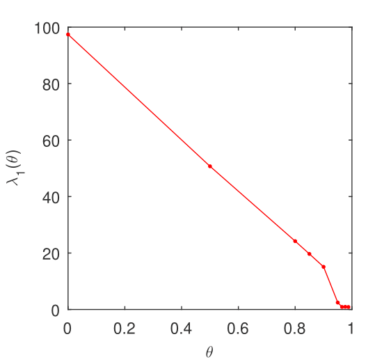
As a validation issue for our computations we have obtained the known value
within an approximation of a thousand.
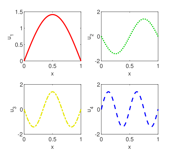
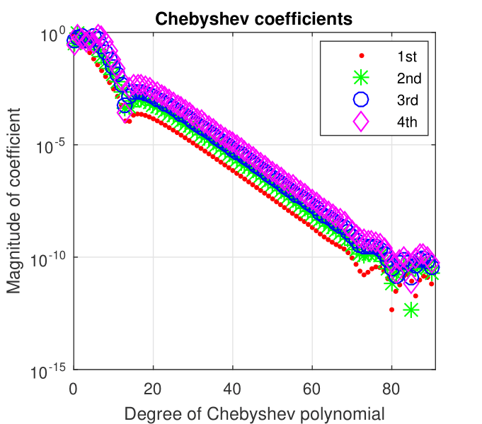
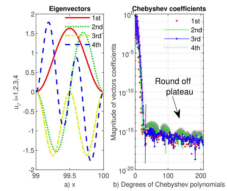
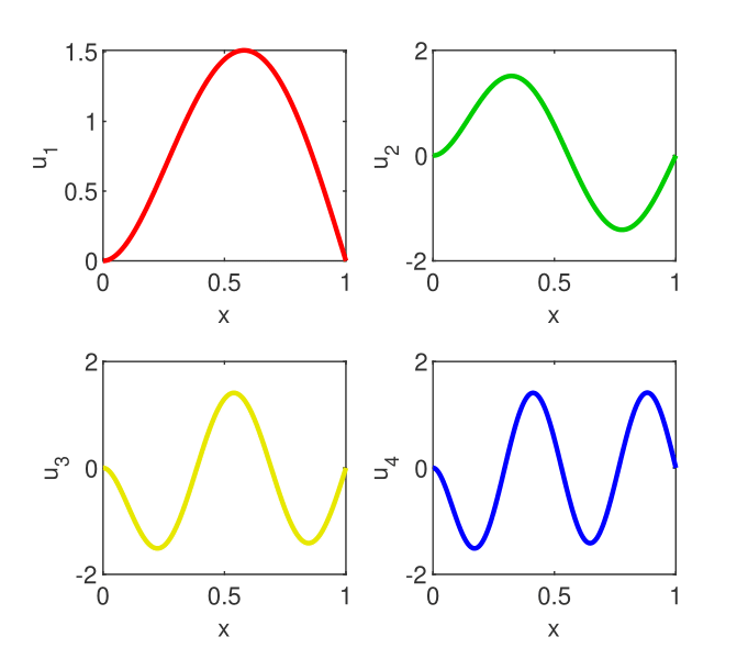
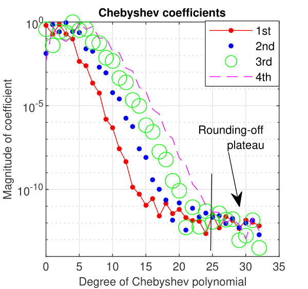
For the highest computable value of parameter we display in Fig. 2 the first four eigenvectors of problem (4) and in Fig. 3 the Chebyshev coefficients of these eigenvectors.
We have to mention that the singularity in the right end becomes more prominent as the tends to . This is confirmed by increasing the degree of the Chebfun approximation. For instance when only a degree Chebyshev polynomial it uses and when the degree of approximation grows to more than (see Fig. 3). It is also worth mentioning that only for growing very close to a truncation of the domain along with the use of the option splitting have been necessary when Chebfun has been used.
4.1.2 The Bénard stability problem
A simplified form of the Bénard stability problem supplied with self-adjoint boundary conditions reads (see for instance GM and LA )
| (5) |
The constant is regarded as a parameter which typically can take the values
All our attempts to solve this problem using Chebfun have failed, so we have resorted to the old strategy.
| according to GM | |||
|---|---|---|---|
Thus we rewrite problem (5) as a homogeneous Dirichlet one attached to a second order differential system, namely
| (6) |
Now we apply to each line the ChC discretization. It leads to the generalized and singular eigenpencil
| (7) |
where the block matrices are defined by
and
The factor in front of comes from the shift of interval to the canonical Chebyshev interval and the matrix signifies the second order Chebyshev differentiation matrix with the homogeneous Dirichlet boundary conditions enforced. The matrices and stand respectively for the identity and zeros matrices of the same dimension as
The following short MATLAB code has been used to solve (6):
N=256;                                    % order of approximation
nu=-(1+4*(pi^2))-sqrt(1+4*(pi^2));        % parameter \nu
[x,D]=chebdif(N,2); D2=D(2:N-1,2:N-1,2);  % differentiation matrices
I=eye(size(D2)); Z=zeros(size(D2));
A=[ 4*D2 -I Z; Z 4*D2 -I; -(nu^2+2*nu+2)*I (nu^2+4*nu+3)*I 4*D2-(2*nu+3)*I];
B=[Z Z Z; Z Z Z; I Z Z];                  % block matrices in pencil
k = 8 ;                                   % number of computed eigs
E=eigs( @(x)(A\(B*x)), size(A,1),k, ’SM’) % Arnoldi method
When the order of approximation is both matrices in (7) have order This tripling of the dimensions of the matrices involved is not a major disadvantage. On the contrary, if we use Henrici’s number as a measure of normality (see for instance our text Cig14 pp. 22-23) we see from the inequality
that matrix is more normal than .
In our previous paper CigJR we have analyzed various methods to solve singular eigenproblems attached to pencils of the form (7). For the problem at hand we have used the Arnoldi method with the MATLAB sequence eigs() and with the above code obtained the eigenvalue reported in Table 1. It is very clear that for the values of considered, the block matrix is non singular and the block matrix is singular and independent of
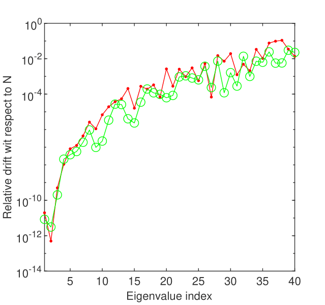
It is extremely important to point out that for the first two values of the parameter in Table 1 our results are very close to those reported in GM . For the other parameter values this no longer happens. A similar situation occurs even for the second eigenvalue. Then, to decide, over the accuracy of our outcomes we resorted to drift. The relative drift, with respect to the order of approximation of the first forty eigenvalues when is displayed in Fig. 4. It suggests that the first two eigenvalues are computed with an accuracy of at least and the first forty with an accuracy of at least . This leads us to believe that we have produced much better approximations for these eigenvalues than those reported in GM as well as LA . Actually, in GM the authors use the SLEUTH code and accept that “it is clear that the code is not very accurate on this problem.”
4.1.3 A self-adjoint eighth-order problem
The eigenproblem of the highest order we consider in this paper is the following
|
|
(8) |
with exact eigenvalues
All our attempts to solve this problem with Chebfun have failed. The abortion message referred to the extremely small conditioning of the eight order Chebyshev collocation differentiation matrix (of the order ).
Instead, the strategy along with ChC worked well and produced vectors from Fig. 5.
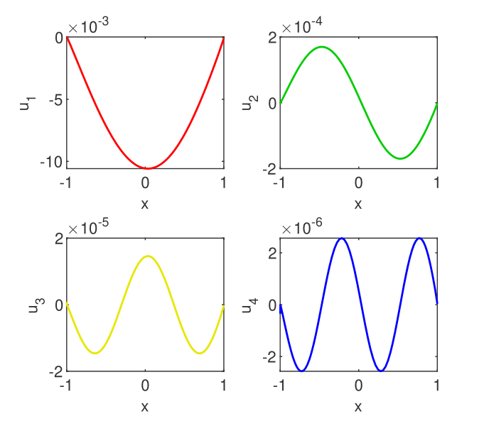
In order to estimate the error with which the eigenvalues were calculated, we display in Fig. 6 b) the relative drift of the first twelve eigenvalues for different approximation orders. Because we know even the exact eigenvalues, we also display the relative errors. It is very clear that the first eigenvalue is computed with better accuracy than . Unfortunately, this means a lower performance by three decimals than that of Magnus expansion reported in Table 10 from PB .
Moreover, this means that we cannot trust more than twelve eigenvalues for this problem.
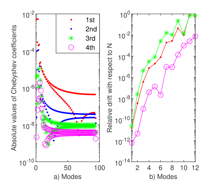
It is clear that ChC along with method has the potential to find the first eigenvalues of a SL problem of arbitrary (even) order with good accuracy. In addition to the Magnus method, this strategy calculates its eigenfunctions (eigenvectors) with reasonable accuracy as can be seen in Fig. 6 a). We use FCT to compute the Chebyshev coefficients of the eigenvectors.
4.2 Clamped boundary conditions
4.2.1 A fourth order problem with a third derivative term
With this first example we have to highlight the importance of preconditioning in improving the accuracy of Chebfun. In the papers HS and GTD , as well as in the monograph Fornberg , the following eigenproblem is carefully studied. It consists of the fourth order differential equation
| (9) |
supplied with the clamped boundary conditions
| (10) |
The eigencondition for this problem is
| (11) |
Problems similar to this appear , for example, in linearized stability analysis in fluid dynamics. In GTD the authors noticed spurious eigenvalues when the problem (9)-(10) is solved by ChT method. These spurious eigenvalues appears in the right-half plane suggesting physical instabilities that do not exist.
The numerical outcomes are displayed in Table 2. Boldfaced digits in the computed eigenvalues show the extent of agreement with the exact values. Thus is very clear that preconditioning Chebfun we can considerably improve its accuracy.
4.2.2 A fourth order eigenproblem from spherical geometry
In GTD the authors consider the eigenproblem
| (12) |
where the operator is defined by
and is a positive integer. They solve this problem by a modified ChT method in order to avoid spurious eigenvalues. We have solved this problem by ChC and obtained for the fist two eigenvalues the numerical values
which agree up to the fourth decimal with the the true values (determined from the eigencondition).
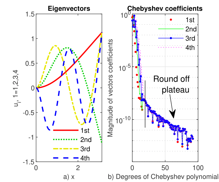
The first four vectors to problem (12) computed by Chebfun are depicted in Fig. 7 a). It is visible that they satisfy the boundary conditions. Their Chebyshev coefficients are displayed Fig. 7 b). About the first twenty coefficients of the first four eigenvectors decrease just as abruptly and smoothly.
4.2.3 A family of sixth order eigenproblems
In FMB the authors consider the following three eigenproblems of sixth order
| (13) |
and introduce an extremely simple modification to the ChT method which eliminates the spurious eigenvalues when such high order eigenproblems are solved.
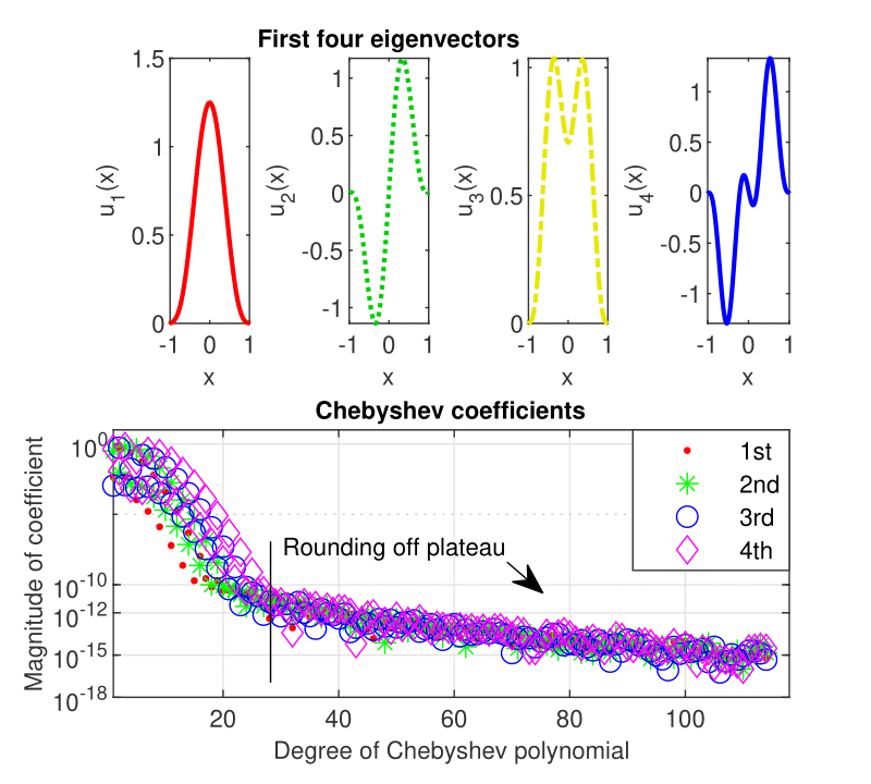
We have tried to solve problem (13) with by Chebfun but all our attempts failed due to the very small conditioning of matrix involved, i.e., around The situation became much better with the preconditioner introduced in Subsection 3.4.
Thus, the first four eigenvectors along with their Chebyshev coefficients are depicted in Fig. 8. As it is apparent from the lower panel of this figure the coefficients of degree up to 30 drop sharply to an absolute value below and then slowly decrease to machine accuracy. This happens at an degree around
The eigenvalues computed by Chebfun agree up to the first three digits with those provided in HS p.405.
4.3 Problems with mixed boundary conditions
4.3.1 The free lateral vibration of a uniform clamped-hinged beam
The fourth order eigenproblem
| (14) |
is considered in Mai and is solved by a non conventional spectral collocation method. In this paper the author shows that the eigenvalues satisfy the transcendental equation
| (15) |
It is extremely important to observe that neither preconditioning nor strategy can handle the mixture of boundary conditions in (14). Thus, this problem tests how well the Chebfun can cope with various boundary conditions.
As the eigenvalues computed from (15) are compared with those obtained by Magnus expansion in PB , we report in Table 3 the latter eigenvalues compared with those provided by Chebfun. A coincidence of at least three decimals can be observed.
| by Chebfun | According to PB | |
|---|---|---|
The first four eigenvectors to problem (14) computed by Chebfun are displayed in Fig. 9. It is perfectly visible that they satisfy the boundary conditions assumed in this problem.
The Chebyshev coefficients of the first four eigenvectors to problem (14) computed by Chebfun are displayed in Fig. 10. They decrease smoothly to somewhere around which is an argument in favor of the accuracy of numerical results.
4.3.2 A fourth order eigenproblem with higher order boundary conditions
In order to show again the Chebfun versatility in introducing boundary conditions we consider the following problem called the cantilevered beam in Euler-Bernouilli theory (see for instance ZWX ). The equation simply reads
| (16) |
and is equipped with the following boundary conditions
| (17) |
The first two boundary conditions state that the beam is clamped in and the last two state that the beam is free in the right hand end. The eigenvalues satisfy the eigencondition
| (18) |
Actually the problem (16)-(17) is self-adjoint. Without going into details we will notice that the first eigenvalue of this eigenproblem is the solution of the minimization problem
where, roughly, is a space of continuous functions satisfying the boundary conditions (17). This Ritz formulation, as well as a weak (variational) formulation can be obtained by multiplying the equation with a function from and a double integration by parts.
Again, these boundary conditions are not treatable by preconditioning or strategy.
| by Chebfun | exact solutions of (18) | |
|---|---|---|
The following simple and short Chebfun code solves the problem (16)-(17).
% Cantilevered beam in Euler-Bernouilli theory
dom=[0,pi];x=chebfun(’x’,dom);   % the domain
L = chebop(dom);
L.op = @(x,y) diff(y,4);         % the operator
L.lbc = @(y)[y; diff(y,1)];        % fixed b. c.
L.rbc = @(y)[diff(y,2); diff(y,3)];% free b. c.
[U,D]=eigs(L,40,’SM’);              % first six eigs.
% Sorted eigenpairs (eigenvalues and eigenvectors)
D=diag(D); [t,o]=sort(D); D=D(o); disp((D.^(1/4)))
U=U(:,o);
In Table 4 are reported the first four eigenvalues computed by Chebfun and by Magnus expansion. A satisfactory agreement is observed.
The first four eigenvectors are displayed in Fig. 11 a) and their Chebyshev coefficients are displayed in the same figure panel b). It is clear that Chebfun uses Chebyshev polynomials of slightly lower degree than and from this level only a sharply decreasing rounding-off plateau follows.
The first four eigenvectors approximating the eigenfunctions are in very good agreement with those exposed in literature. Using the definition of the scalar product of two vectors and , namely , we can easily check the orthonormality of eigenvectors.
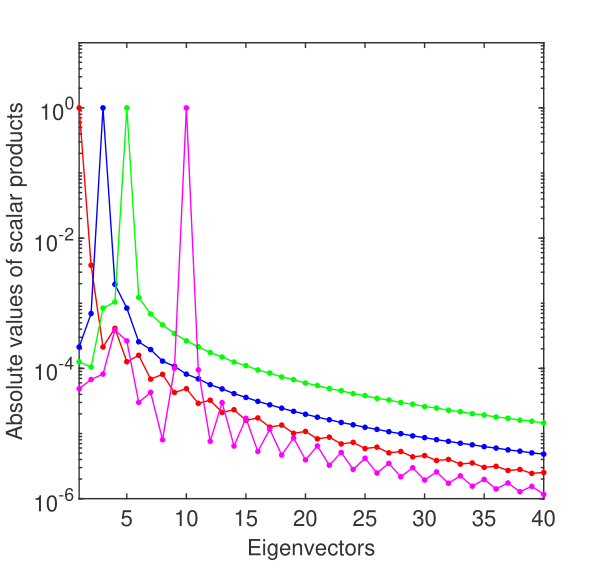
The curves in Fig. 12 clearly shows that the eigenvectors of this problem computed by Chebfun are orthonormal.
4.3.3 The harmonic oscillator and its second and third powers.
We wanted to test our strategy on a problem whose differential equation exhibits stiffness in at least part of the range. Thus, along with the well known harmonic oscillator operator
we have considered its second and third powers, namely
and
Actually we want to solve the fourth order eigenvalue problem for namely
| (19) |
and the sixth order eigenvalue problem
| (20) |
corresponding to the cube of the harmonic oscillator operator. The eigenvalues of the harmonic oscillator are and those of and are the second and the third powers respectively of According to the definition for classification of SL problems, given in this Section 2, the eigenproblems (19) and (20) are singular.
We have to observe that no boundary conditions are needed because the problem is of limit-point type Everitt : the requirement that the eigenfunctions be square integrable suffices as a boundary condition. In GM the problem (20) is solved by a SLEUTH code along with domain truncation. Actually the authors truncate this problem to the interval , and impose the simplest boundary conditions at Along with these boundary conditions the eigenproblem becomes self-adjoint.
The first four eigenvectors of the cube of harmonic oscillator computed by SiC are displayed in the upper panels of Fig. 13. Their sinc coefficients are displayed in the lower panel of the same figure. Roughly speaking it guarantees us an accuracy of at least in the computation of these eigenvectors.
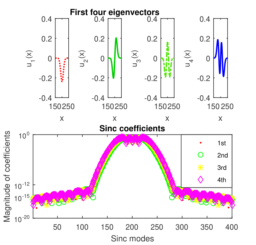
SiC computes the integers with an accuracy of at least six digits.
The relative drift, with respect to of the first eigenvalues of the cube of harmonic oscillator computed by SiC are displayed in Fig. 14 a). It tells us that the first eigenvalues are “good”within an accuracy of approximately It means the "highest" confirmation of the Eigenvalues-Rule-of-Thumb formulated by Boyd (see Sect. 3.3).
Trying to explain this spectacular phenomenon we cannot forget the fact that the derivation matrices of SiC are symmetric. This leads to normal matrices (operators) whose eigenpairs are properly computable.
If we compare this result with Table 10 from GM , where the best accuracy in computing of the first eigenvalue is , we can speak of a total superiority of SiC method over SLEUTH.
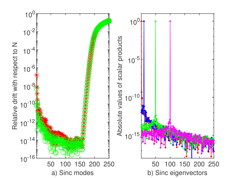
In Fig. 14 b) in a log-linear plot we display the scalar product of some eigenvectors. They prove that the SiC computed eigenvectors are indeed orthonormal. This means that we can trust at least the first eigenpairs computed by SiC. The following few lines of MATLAB compute the above eigenpairs:
% The sinc differentiation matrices [Weideman & Reddy]
N=400;M=6;h=0.1; %Orders of approximation and differentiation and scaling factor
[x, D] = sincdif(N, M, h); D1=D(:,:,1);D2=D(:,:,2);D6=D(:,:,6);
% The cube of the "harmonic oscillator" operator
L=-D6+D2*(3*diag(x.^2)*D2)+D1*(diag(8-3*(x.^4))*D1)+diag(x.^6-14*(x.^2));
% Finding eigenpairs of L
[U,S]=eigs(L,250,0); S=diag(S); [t,o]=sort(S); S=S(o);
Unfortunately, Chebfun along with domain truncation fails in solving the sixth order problem (20) with or without preconditioning. Actually, a warning concerning the very bad conditioning of the matrix is issued.
However, Chebfun behaves fairly well in solving the fourth order problem (19), i.e., computes the corresponding integers with the same accuracy as SiC. We have solved the equation (19) on the truncated interval for various along with the boundary conditions
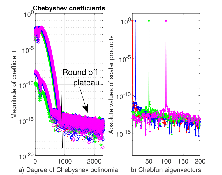
The Chebyshev coefficients of the first four eigenvectors of eigenproblem (19) computed by Chebfun are displayed in Fig. 15 a). An important aspect must be highlighted, namely the first about polynomial coefficients decrease steeply and smoothly to about after which up to the order of follows a wide rounding-off plateau.This is the polynomial of the highest degree that Chebfun has used in our numerical experiments. The curves in Fig. 15 b) show the orthonormality of Chebfun eigenvectors.
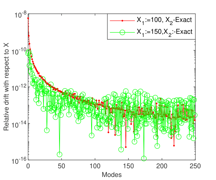
The relative drift with respect to the length of integration interval of the first eigenvalues to problem (19), when it is solved by Chebfun, is displayed in Fig. 16. It means that the numerical stability is lost for length larger than and a set of small eigenvalues can be computed with an accuracy better than .
5 Conclusions and open problems
After analyzing these challenging problems, some firm conclusions can be drawn.
First of all, Chebfun can easily handle any type of boundary condition. This is a significant advantage. Thus, for fourth order eigenproblems, the direct application of Chebfun is versatile in handling various high order boundary conditions and produces reliable outcomes. Furthermore, for problems with clamped boundary conditions both methods, Chebfun as well as ChC, improve their results with at least two, three decimals by preconditioning.
For sixth order eigenproblems, the Chebfun situation is not so encouraging. Its direct application is very uncertain. Matrices whose conditioning order drops to appear, which most often lead to inaccurate results. For problems of this order or more, subjected to hinged boundary conditions, the reduction to second-order systems and then the application of the ChC method is the best strategy. In this way we managed to establish a conjecture for the Viola’s problem regarding its lowest eigenvalue.
For fourth order problems on the real line Chebfun along with the truncation of the domain worked fairly well as was the case with the second power harmonic oscillator. As an absolute novelty, we have established in this case the numerical stability with respect to the length of the integration interval. Instead, for the sixth order eigenproblems on the real line the SiC method remains the unique feasible alternative.
In fact, this method is the best in the sense that we can trust the first half of computed eigenpairs. To our knowledge, no software package has reached this performance so far.
As an open problem remains that of finding preconditioning methods for the case of hinged boundary conditions or some other types of boundary conditions.
This paper comes shortly after in another one (see Cig21 ) we have approached, with the same two classes of methods, singular Schröedinger eigenproblems. In this situation we can appreciate that, ChC along with Chebfun, are a better alternative in some respects to other existing methods for a very wide range of eigenproblems. Both compute eigenvectors (approximating eigenfunctions) and by drift estimation demonstrate numerical stability. In addition, the drift with respect to shows the degree of accuracy up to which a set of eigenvalues is computed. The situation when both types of methods can be applied to the same problem is the ideal one and the one that produces the safest results.
Conflicts of interest: The author declares no conflict of interest.
Sample availability: Samples of the Chebfun codes are available from the author by request.
Abbreviations: The following abbreviations are used in this manuscript:
| ChC | Chebyshev collocation method |
|---|---|
| ChT | Chebyshev tau method |
| strategy to reduce a 2nth-order equation to a second order system | |
| FCT | fast Chebyshev transform |
| FD | finite difference method |
| FE | finite element method |
| MATSLISE | a MATLAB package for the numerical solution of SL and Schröedinger equations |
| SiC | sinc spectral collocation |
| SL | Sturm-Liouville |
| SLEDGE | Sturm-Liouville estimates determined by global errors |
| SLEUTH | Sturm-Liouville Eigenvalues using Theta Matrices |
References
- (1) Straughan, B.: Stability of Wave Motion in Porous Media, Springer Science+Business Media, LLC 2008
- (2) Trefethen, L.N., Birkisson, A., Driscoll, T. A. Exploring ODEs. SIAM, Philadelphia, US, 2018
- (3) Pruess, S., Fulton, C. T. Mathematical Software for Sturm-Liouville Problem. ACM T. Math. Software 1993, 19, 360–376.
- (4) Pruess, S., Fulton, C. T., Xie, Y. An Asymptotic Numerical Method for a Class of Singular Sturm-Liouville Problems. ACM SIAM J. Numer. Anal. 1995 32, 1658–1676.
- (5) Marletta, M., Pryce, J.D. LCNO Sturm-Liouville problems. Computational difficulties and examples. Numer. Math. 1995, 69, 303–320.
- (6) Pryce, J.D., Marletta, M. A new multi-purpose software package for Schrödinger and Sturm–Liouville computations. Comput. Phys. Comm. 1991, 62, 42–54.
- (7) Bailey, P. B., Everitt, W. N., Zettl, A. Computing Eigenvalues of Singular Sturm-Liouville Problems. Results Math. 1991, 20, 391–423.
- (8) Bailey, P.B., Garbow, B., Kaper, H., Zettl, A. Algorithm 700: A FORTRAN software package for Sturm-Liouville problems. ACM T. Math. Software. 1991, 17, 500–501.
- (9) Ledoux, V., Van Daele, M., Vanden Berghe, G. MATSLISE: A MATLAB Package for the Numerical Solution of Sturm-Liouville and Schrödinger Equations. ACM T. Math. Software. 2005, 31, 532–554.
- (10) Baeyens, T., Van Daele, M. The fast and accurate computation of eigenvalues and eigenfunctions of time-independent one-dimensional Schrödinger equations. Comput. Phys. Comm. 2021, 258 https://doi.org/10.1016/j.cpc.2020.107568
- (11) Abbasbandy, S., Shirzadi, A. A new application of the homotopy analysis method: Solving the Sturm–Liouville problems. Commun. Nonlinear. Sci. Numer. Simulat. 2011, 16, 112–-126.
- (12) Perera, U.; Böckmann, Ch. Solutions of Direct and Inverse Even-Order Sturm-Liouville Problems Using Magnus Expansion. Mathematics 2019, 7, 544; . https://doi.org/10.3390/math7060544
- (13) Gheorghiu, C.I. Spectral Methods for Non-Standard Eigenvalue Problems. Fluid and Structural Mechanics and Beyond. Springer-Verlag, Cham Heidelberg New-York Dondrecht London, 2014
- (14) Greenberg, G., Marletta, M. Oscillation Theory and Numerical Solution of Sixth Order Sturm-Liouville Problems. SIAM J. Numer. Anal. 1998, 35, 2070-2098.
- (15) Everitt, W.N. A Catalogue of Sturm-Liouville Differential Equations. In Sturm-Liouville theory: Past and Present; Amrein, W. O., Hinz, A. M., Hinz, D. B., Eds. Birkhäuser Verlag Basel/Switzerland, 2005; pp.271–331.
- (16) Driscoll, T. A., Bornemann, F., Trefethen, L.N. The CHEBOP System for Automatic Solution of Differential Equations. BIT 2008, 48, 701–723.
- (17) Driscoll, T. A., Hale, N., Trefethen, L.N. Chebfun Guide. Pafnuty Publications, Oxford, UK 2014
- (18) Driscoll, T. A., Hale, N., Trefethen, L.N. Chebfun-numerical computing with functions. http://www.chebfun.org. Accessed 15 November 2019
- (19) Gheorghiu, C.I. Spectral Collocation Solutions to Problems on Unbounded Domains. Casa Cărţii de Ştiinţă Publishing House, Cluj-Napoca, Romania 2018
- (20) Weideman, J. A. C., Reddy, S. C. A MATLAB Differentiation Matrix Suite. ACM T. Math. Software 2000, 26, 465–519. 26, 465–519
- (21) Gheorghiu, C.I., Pop, I.S. A Modified Chebyshev-Tau Method for a Hydrodynamic Stability Problem. In Proceedings of the International Conference on Approximation and Optimization; Stancu,D.D., Coman, Gh., Breckner, W. W., Blaga, P., Eds.; Transilvania Press: Cluj-Napoca, Romania, Volume II, 1996; pp. 119–126.
- (22) Boyd, J. P. Traps and Snares in Eigenvalue Calculations with Application to Pseudospectral Computations of Ocean Tides in a Basin Bounded by Meridians. J. Comput. Phys. 1996, 126, 11–20.
- (23) Gheorghiu, C.I. Accurate Spectral Collocation Computation of High Order Eigenvalues for Singular Schrödinger Equations. Computation 2021, 9, 2. https://doi.org/10.3390/computation9010002
- (24) Boyd, J. P. Chebyshev and Fourier Spectral Methods. Dover Publications, New-York, US, 2000; pp. 127–158
- (25) Huang, W., Sloan, D.M. The Pseudospectral Method for Solving Differential Eigenvalue Problems. J. Comput. Phys. 1994, 111, 399–409.
- (26) Straughan, B. The Energy Method, Stability, and Nonlinear Convection, Springer-Verlag, New-York, lnc. 1992; pp. 218–222.
- (27) Lesnic, D., Attili, S. An Efficient Method for Sixth-order Sturm-Liouville Problems. Int. J. Sci. Technol. 2007, 2, 109–114.
- (28) Gheorghiu, C.I., Rommes, J. Application of the Jacobi-Davidson method to accurate analysis of singular linear hydrodynamic stability problems. Int. J. Numer. Meth. Fluids 2013, 71, 358–369.
- (29) Gardner, D.R., Trogdon, S.A., Douglass, R.W. A Modified Spectral Tau Method That Eliminates Spurious Eigenvalues. J. Comput. Phys. 1989, 80, 137–167.
- (30) Fornberg. B. A practical guide to pseudospectral methods. Cambridge University Press, Cambridge, UK, 1998; pp.89–90
- (31) McFadden, G.B., Murray, B.T., Boisvert, R.F. Elimination of Spurious Eigenvalues in the Chebyshev Tau Spectral Method. J. Comput. Phys. 1990, 91, 228–239.
- (32) Mai-Duy, N. An effective spectral collocation method for the direct solution of high-order ODEs. Commun. Numer. Methods Eng. 2006, 22, 627–-642.
- (33) Zhao, S.; Wei, G.W.; Xiang,Y. DSC analysis of free-edged beams by an iteratively matched boundary method. J. Sound. Vib. 2005, 284, 487–-493.
1. Straughan, B., Stability of Wave Motion in Porous Media, Springer Science+Business Media: New York, NY, USA, 2008.
2. Trefethen, L.N., Birkisson, A.; Driscoll, T.A., Exploring ODEs; SIAM: Philadelphia, PA, USA, 2018.
3. Pruess, S., Fulton, C.T., Mathematical Software for Sturm-Liouville Problem. ACM Trans. Math. Softw. 1993, 19, 360–376.
4. Pruess, S., Fulton, C.T., Xie, Y., An Asymptotic Numerical Method for a Class of Singular Sturm-Liouville Problems. ACM SIAM J. Numer. Anal. 1995, 32, 1658–1676.
5. Marletta, M., Pryce, J.D., LCNO Sturm-Liouville problems. Computational difficulties and examples. Numer. Math. 1995, 69, 303–320.
6. Pryce, J.D., Marletta, M., A new multi-purpose software package for Schrödinger and Sturm–Liouville computations. Comput. Phys. Comm. 1991, 62, 42–54.
7. Bailey, P.B., Everitt, W.N., Zettl, A., Computing Eigenvalues of Singular Sturm-Liouville Problems. Results Math. 1991, 20, 391–423.
8. Bailey, P.B., Garbow, B., Kaper, H., Zettl, A., Algorithm 700: A FORTRAN software package for Sturm-Liouville problems. ACM Trans. Math. Softw. 1991, 17, 500–501.
9. Ledoux, V.,Van Daele, M., Vanden Berghe, G., MATSLISE: A MATLAB Package for the Numerical Solution of Sturm-Liouville and Schrödinger Equations. ACM Trans. Math. Softw. 2005, 31, 532–554.
10. Baeyens, T., Van Daele, M., The Fast and Accurate Computation of Eigenvalues and Eigenfunctions of Time-Independent One-Dimensional Schrödinger Equations. Comput. Phys. Commun. 2021, 258, 107568, doi:10.1016/j.cpc.2020.107568.
11. Abbasb, Y.S., Shirzadi, A., A new application of the homotopy analysis method: Solving the Sturm—Liouville problems. Commun. Nonlinear. Sci. Numer. Simulat. 2011, 16, 112—126.
12. Perera, U., Böckmann, C., Solutions of Direct and Inverse Even-Order Sturm-Liouville Problems Using Magnus Expansion. Mathematics 2019, 7, 544, doi:10.3390/math7060544.
13. Gheorghiu, C.I., Spectral Methods for Non-Standard Eigenvalue Problems: Fluid and Structural Mechanics and Beyond; Springer: Heidelberg, Germany, 2014.
14. Greenberg, G., Marletta, M., Oscillation Theory and Numerical Solution of Sixth Order Sturm-Liouville Problems. SIAM J. Numer. Anal. 1998 35, 2070–2098.
15. Everitt, W.N., A Catalogue of Sturm-Liouville Differential Equations. In Sturm-Liouville theory: Past and Present; Amrein, W.O., Hinz, A.M., Hinz, D.B., Eds.; Birkhäuser Verlag: Basel, Switzerland, 2005; pp. 271–331.
16. Driscoll, T.A., Bornemann, F., Trefethen, L.N., The CHEBOP System for Automatic Solution of Differential Equations. BIT 2008, 48, 701–723.
17. Driscoll, T.A., Hale, N., Trefethen, L.N., Chebfun Guide; Pafnuty Publications: Oxford, UK, 2014.
18. Driscoll, T.A., Hale, N., Trefethen, L.N., Chebfun-Numerical Computing with Functions. Available online: http://www.chebfun. org (accessed on 15 November 2019).
19. Gheorghiu, C.I., Spectral Collocation Solutions to Problems on Unbounded Domains; Casa Cartii de ¸Stiinta Publishing House: ClujNapoca, Romania, 2018.
20. Weideman, J.A.C.; Reddy, S.C., A MATLAB Differentiation Matrix Suite. ACM Trans. Math. Softw. 2000, 26, 465–519.
21. Gheorghiu, C.I., Pop, I.S., A Modified Chebyshev-Tau Method for a Hydrodynamic Stability Problem. In Proceedings of the International Conference on Approximation and Optimization; Stancu, D.D., Coman, G., Breckner, W.W., Blaga, P., Eds.; Transilvania Press: Cluj-Napoca, Romania, 1996; Volume II, pp. 119–126.
22. Boyd, J.P., Traps and Snares in Eigenvalue Calculations with Application to Pseudospectral Computations of Ocean Tides in a Basin Bounded by Meridians. J. Comput. Phys. 1996, 126, 11–20.
23. Gheorghiu, C.I,. Accurate Spectral Collocation Computation of High Order Eigenvalues for Singular Schrödinger Equations. Computation 2021, 9, 2. doi:10.3390/computation9010002.
24. Boyd, J.P., Chebyshev and Fourier Spectral Methods; Dover Publications: New York, NY, USA, 2000; pp. 127–158.
25. Huang, W., Sloan, D.M., The Pseudospectral Method for Solving Differential Eigenvalue Problems. J. Comput. Phys. 1994, 111, 399–409.
26. Straughan, B., The Energy Method, Stability, and Nonlinear Convection; Springer: New York, NY, USA, 1992; pp. 218–222.
27. Lesnic, D., Attili, S., An Efficient Method for Sixth-order Sturm-Liouville Problems. Int. J. Sci. Technol. 2007, 2, 109–114.
28. Gheorghiu, C.I., Rommes, J., Application of the Jacobi-Davidson method to accurate analysis of singular linear hydrodynamic stability problems. Int. J. Numer. Meth. Fluids 2013, 71, 358–369. doi:10.1002/fld.3669.
29. Gardner, D.R., Trogdon, S.A., Douglass, R.W., A Modified Spectral Tau Method That Eliminates Spurious Eigenvalues. J. Comput. Phys. 1989, 80, 137–167.
30. Fornberg, B., A Practical Guide to Pseudospectral Methods; Cambridge University Press: Cambridge, UK, 1998; pp. 89–90.
31. McFadden, G.B.; Murray, B.T.; Boisvert, R.F., Elimination of Spurious Eigenvalues in the Chebyshev Tau Spectral Method. J. Comput. Phys. 1990, 91, 228–239.
32. Mai-Duy, N., An effective spectral collocation method for the direct solution of high-order ODEs. Commun. Numer. Methods Eng. 2006, 22, 627–642.
33. Zhao, S., Wei, G.W., Xiang, Y., DSC analysis of free-edged beams by an iteratively matched boundary method. J. Sound. Vib. 2005, 284, 487–493.