Abstract
The self-correlation (SC) method proposed three decades ago by Percy, Jakate and Matthews is a complementary time series analysis method which provides a characterization of a variability phenomenon and an estimation of the involved time-scale. It can be applied to periodic, quasi-periodic and irregular phenomena, for either evenly or unevenly sampled data. An important deficiency of this method – mentioned by Percy himself – is the fact that the statistical properties of the SC are unknown so that the statistical significance of an ‘observed’ (quasi-)periodicity cannot be estimated.
In this paper, we investigate analytically and numerically the properties of the SC of a harmonic periodic signal by taking into account the influence of the finite length of the data set, the non-equidistant sampling, and the presence of an additive Gaussian white noise. This method is used to investigate the already inferred periodic modulation of the orbital period of the eclipsing binary system ER Vul.
In addition, we propose an improvement of the SC method by applying the ‘stacking method’ already used in seismology, which we call the enhanced SC (ESC) method. A statistical test relying on the ESC method together with Monte Carlo simulations allow us to claim the presence of a deterministic component at a significantly higher confidence level than that obtained through a Fourier based method.
The evaluation of the detectability of the ER Vul periodic phenomenon through the ESC method provides similar results as those previously obtained using the Fourier based method.
Authors
M. Crăciun
-Tiberiu Popoviciu Institute of Numerical Analysis, Romanian Academy
C. Vamoș
-Tiberiu Popoviciu Institute of Numerical Analysis, Romanian Academy
A. Pop
Keywords
Cite this paper as:
M. Crăciun, C. Vamoş, A. Pop, Detection of low level periodic signals through enhanced self-correlation method. The case of ER Vulpeculae, Monthly Notices of the Royal Astronomical Society, 448, 2066-2076 (2015)
DOI: 10.1093/mnras/stv108.
References
see the expansion block below.
About this paper
Publisher Name
Oxford Academic
Print ISSN
0035-8711
Online ISSN
1365-2966
MR
?
ZBL
?
Detection of low level periodic signals through enhanced self-correlation method. The case of ER Vulpeculae
Abstract
The self-correlation (SC) method proposed three decades ago by Percy, Jakate and Matthews is a complementary time series analysis method which provides a characterisation of the variability phenomenon and an estimation of the involved time scale. It can be applied to periodic, quasiperiodic and irregular phenomena, for either evenly or unevenly sampled data. An important deficiency of this method – mentioned by Percy himself – is the fact that the statistical properties of the SC are unknown so that the statistical significance of an ‘observed’ (quasi)periodicity can not be estimated. In this paper, we investigate analytically and numerically the properties of the SC of a harmonic periodic signal by taking into account the influence of the finite length of the data set, the non-equidistant sampling, and the presence of an additive Gaussian white noise. This method is used to investigate the already inferred periodic modulation of the orbital period of the eclipsing binary system ER Vul. In addition, we propose an improvement of the SC method by applying the ‘stacking method’ already used in seismology, which we call the enhanced SC (ESC) method. A statistical test relying on the ESC method together with Monte Carlo simulations allow us to claim the presence of a deterministic component at a significantly higher confidence level than that obtained through a Fourier based method. The evaluation of the detectability of the ER Vul periodic phenomenon through the ESC method provides similar results as those previously obtained using the Fourier based method.
keywords:
methods: data analysis - methods: statistical - stars: individual: ER Vulpeculae1 Introduction
In many cases, the detection of periodic signals in astronomical time series may be a difficult task due to the low number of available observations with an uneven sampling, to the existence of large gaps, or to the high level of noise. In such cases the amplitude spectrum analysis can be supplemented with Monte Carlo simulations in order to estimate the statistical significance of the highest peak [see e.g. Kuschnig et al. (1997); Pop et al. (2010) and references therein]. Assuming that the values of the parameters of the detected signal are those estimated through the nonlinear least-squares method [see e.g. Pop (1996, 1999)], an estimation methodology of the detectability of the detected periodic signal was also proposed (Pop & Vamoş, 2013). It relies on two different Monte Carlo simulations, each of them treated both through frequentist and Bayesian approaches.
A conceptually different analysis method which can be applied to such astronomical time series is the self-correlation (SC) method proposed by Percy et al. (1981) [see also Percy et al. (1993, 2003)]. Although it is an autocorrelation method, it must not be confused with the classical autocorrelation function. As Percy and his collaborators mentioned, the SC analysis ‘measures the cycle-to-cycle behaviour of the star averaged over all the data’ [e.g. Percy et al. (2006a); Percy & Palaniappan (2006)]. According to Percy et al. (2006a) the method “does not have the equivalent of the ‘aliasing’ problem found in the Fourier analysis” [see also Percy et al. (1993, 2002, 2003); Percy (2007) and Marinova & Percy (1999)]. Consequently, it was found to be useful in conjunction with the visual inspection of the light curves and the Fourier analysis in case of data displaying some degree of irregularity and having regular gaps of the same order of magnitude as the length of the involved (quasi)period in order to distinguish between true and alias periods [e.g. Percy et al. (1993, 2002, 2003, 2006a, 2006b, 2010); Percy & Mohammed (2004)].
The SC is defined as the average absolute value of the variations over a given time lag of a time series. If the time series is periodic with the period , then its variation for lags equal to the multiples of vanishes and the SC reaches a minimum. If the periodic component is hidden in noise, then the shape of SC is distorted, but the positions of its minima can supply useful information concerning the respective periodicity. For example, Percy et al. (1993) noted that the level of the SC minima is the observational scatter of the data, while that of the maxima is related to the amplitude of the periodic signal in the observational data. In addition, the SC method has the desirable property to be suitable for the analysis of time series arising from quasiperiodic and irregular phenomena.
Unlike the amplitude/power spectrum analysis, the SC method allows to perform the signal detection not in frequency domain, but in the time domain. The presence of a periodic component is signaled not by a single peak, but by a series of minima which are approximately equidistant. Depending on the length of the analysed time series and on the involved periodicity, it is possible to use more than one minimum in order to perform the periodicity detection.
The present paper has two main goals. First, we want to remove an important deficiency of the SC method already outlined by Percy et al. (2006a): the lack of information concerning the statistical significance of a periodicity or of a time scale detected using the SC function. The second goal is to prove the power of this method in the case of pathological data sets on variable stars featured by low number of unevenly sampled observations in the presence of a high noise level. We propose an improvement of the SC method by thickening the grid on which the SC is computed. Using it in Monte Carlo simulations we significantly improve the false alarm probability which allow us to claim the detection of the deterministic component in a noisy time series.
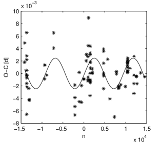
As an application we consider the orbital period variability of the eclipsing binary system ER Vulpeculae investigated in a recent paper by Pop & Vamoş (2013) for which contradictory results were obtained by different researchers. After rejecting some outlying points and averaging those corresponding to the same events, they obtained a data set consisting in 91 times of minimum light which cover a relatively short time base of 54.9 yr (Fig. 1). They found that the run of the residuals can be described by a statistically significant secular parabolic trend corresponding to a relatively slow increasing trend in the orbital period featured by a relative period change rate of yr-1, and a 17.78 yr periodic component, with a low amplitude of about 3.5 min.
The confidence level for the rejection of the null hypothesis that there is no periodic component in the ER Vul time series was a little over 96 per cent, smaller than the threshold usually taken into account (99.9 per cent). Using an improved SC algorithm, the enhanced self-correlation (ESC), we have obtained a confidence level of 99.98 per cent for the existence of a deterministic component of the variability phenomenon of ER Vul, much higher than that previously estimated for a periodic component by Pop & Vamoş (2013). The evaluation of the detectability of the above inferred periodicity supplied somewhat worse results with respect to those estimated by Pop & Vamoş (2013). However, the relatively good coincidence between the results of the analyses performed through two complementary methods is interpreted by us as a confirmation of the detection of the periodic modulation of the orbital period of the eclipsing binary ER Vul. It represents both an important step in understanding this system and an insight into the involved physical phenomena. Obviously, this result needs future confirmation relying on higher quality observational data.
2 The self-correlation function and its basic properties
In this section we analyse the properties of the SC function for some particular cases in which we gradually introduce the characteristics of an observed astronomical time series, like that of ER Vul. First of all, we analytically study the SC function for a continuous sinusoid. After that, we numerically study its discretization both on equidistant and nonequidistant grids. Finally, we analyse the influence of a superposition of a Gaussian white noise on this deterministic signal.
2.1 Deterministic continuous function of time
For the sake of clarity, we define the SC function for the ideal case of a continuous function defined on a finite interval . For a positive time lag , the self-correlation is the average absolute value of the function variation
| (1) |
A general conclusion drawn from this definition is: if is a periodic function with the period , then for the integrant vanishes and for any integer . Therefore, the zeros of the function are separated by distances equal to the period , between which has positive values. Hence the graph of is a succession of humps limited by its zeros. The positions and values of the maxima and minima can be used to identify a periodic component within a real time series.
The derivation of the properties of the SC function for an arbitrary function is difficult and we analyse only a simple case which is of interest from practical viewpoint. We consider a periodic harmonic signal , where is the frequency, is the amplitude, and the period is If the definition domain is infinite , then Eq. (1) gives
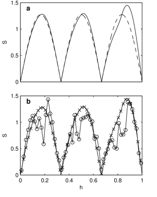
for any (Appendix A). In this case the SC function has the same period as and, in accordance with the general properties of SC, the minima of are equal to zero and occur at integer multiples of the period . The maxima are equal to and are situated at odd multiples of the half-period . In Fig. 2a we plot with dashed line for and . This frequency is similar to that of the estimated periodic component of the curve of ER Vul in Fig. 1 (Pop & Vamoş, 2013).
Real time series have finite lengths and we want to study the effect of a finite definition domain in the previous ideal case. If we limit the continuous sinusoid to the interval , then has a more intricate analytic formula
| (2) | |||||
where , and is the integer part function (Appendix A). In Figs. 2a and b the graph of for is plotted with continuous line. One notices that the SC of a finite signal is no more periodic due to the variation of the integration interval as a function of in Eq. (1). The humps are distorted and unequal, especially the last one. (A more detailed analysis of the graph of is given in Appendix A).
2.2 Discrete time series
The next idealization that we remove is the continuity of the signal. Let us consider an arbitrary time series , resulted from the observation of a variability phenomenon. The SC function of such a time series has discrete values and is computed numerically. The numerical algorithm for the computation of SC must be a discretization of the definition (1).
We can use the following algorithm given by Percy et al. (1981, 1993, 2002, 2003, 2006a, 2006b); Percy & Sen (1991); Percy & Mohammed (2004); Percy & Palaniappan (2006):
- i.
-
For all we compute the differences and , where .
- ii.
-
The differences are sorted in the ascending order of their corresponding values.
- iii.
-
The interval containing all the differences is divided in bins of length . We denote the grid points with and with the interval .
- iv.
-
The value of the self-correlation function for each interval is
(3) where is the number of values within the interval . Unlike the case of continuous function where the values of the SC function are denoted with , we denote the discrete values of the SC function with .
The result of the application of this algorithm depends on the choice of the computation grid, i.e. on the parameters and which are linked through the relation Consequently, only one of these parameters must be fixed. There are some empiric criteria for this choice. We denote by the characteristic time of the signal contained by the analysed time series. If the signal is not quasiperiodic, but periodic, then . The observed time series has to contain between to characteristic time intervals (Percy et al., 2004). According to the ‘rule of thumb’ mentioned by Percy and his collaborators, in order to obtain a statistically significant value of , it must be obtained by averaging at least values of in each bin (Percy et al., 2002, 2003; Percy & Mohammed, 2004; Percy et al., 2006a, b). It is also desirable to have at least values of on an interval equal to , i.e. such that the shape of the SC is described with an acceptable resolution.
In order to check the numerical algorithm for the computation of we apply it to the time series with discretized on an equidistant grid with . This is the discretization of the continuous sinusoid defined for and analysed in Section 2.1. In Fig. 2b one can see that for , the values of (represented with cross markers) approximate very well the theoretical values. We conclude that the discretization on an equidistant grid does not distort the shape of .
Very often the astronomical time series have an uneven sampling as in the case of ER Vul (Fig. 1). In order to analyse the influence of an uneven sampling on the SC, we have calculated the self-correlation with of the same sinusoid (), but discretized on the time grid of ER Vul rescaled to the interval (Fig. 2b). We notice that in this case:
- i.
-
In the region of maxima the shape of the SC function is strongly distorted and due to the non-equidistant grid, large fluctuations occur, even if the signal is periodic.
- ii.
-
In the other regions agrees quite well with calculated theoretically for the finite signal (Eq. 2).
- iii.
-
The minima positions are the same for an equidistant grid, even if their level is not equal to zero. In fact, the minima of the SC function vanish for an equidistant grid, only if its step is a divisor of the signal period.
The fact that neither the positions, nor the shape near the minima are modified by the non-equidistant grid, justifies their use to estimate the period of a deterministic component possibly present in observational data.
2.3 Noisy discrete time series
Astronomical time series are always more or less affected by noise, as in the case of ER Vul. We begin the study of the influence of the observational noise on the SC by considering a time series consisting of Gaussian white noise only. If for any the values are normally distributed with zero mean and standard deviation , then the differences are also normally distributed, but with the standard deviation and their average absolute value is independent of and
| (4) | |||||
Then the average of SC given by Eq. (3) is for any value of and it does not depend on the type of the temporal grid.
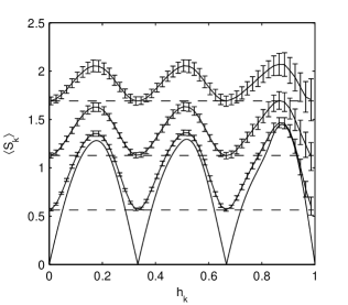
If the time series consists of a superposition of a periodic function and a Gaussian white noise, the average can not be computed theoretically. We have generated statistical ensembles of 1000 artificial time series obtained by superposing Gaussian white noises with a given standard deviation over the previously analysed periodic signal. For each artificial time series consisting of equidistant data we have numerically computed the SC function, and then, for each bin (), we have calculated the average value and its standard deviation (Fig. 3).
From the results of these simulations we draw the following conclusions:
- i.
-
The positions of minima and maxima of remain the same as in the case of the periodic signal without the additive noise.
- ii.
-
The average level of the minima is equal to the value obtained for Gaussian white noise, the contribution of the deterministic part vanishing. This property is valid only for the average , the values of an individual displays significant fluctuations around the average value. Thus, we have obtained the rigorous formulation of the empiric observations that the minima level of the SC function is approximately equal to the average deviation of the noise existing in the analysed time series (Percy et al., 1993, 2002, 2003; Percy & Mohammed, 2004; Percy et al., 2006a, b; Percy & Palaniappan, 2006; Percy & Long, 2010).
- iii.
-
The level of maxima of increases when the standard deviation of the noises increases, but less than the level of minima.
- iv.
-
The difference between the maxima and minima (the peak-to-peak amplitude) of decreases when increases following a power law. At the limit, when the contribution of the periodic signal to the time series is negligible, becomes constant, as in the case of the Gaussian white noise.
- v.
-
The standard deviation of (represented in Fig. 3 with error bars) increases when and the standard deviation of the noise increase.
From all the cases presented in this section it follows that the minima of preserve their equidistant distribution in case of realistic time series allowing the estimation of the period of the periodic component as the mean average distance between the consecutive minima in the SC (Percy et al., 2002, 2003; Percy & Mohammed, 2004; Percy & Palaniappan, 2006). However, it is possible that the minima occurring for large values of the time lag are strongly distorted at high noise levels. In the following section we present a method allowing us to establish those extrema of the SCD which can be used to estimate the deterministic component even in such cases. This is an extension of the SC method which was till now used especially for time series with low noise level.
3 Enhanced self-correlation (ESC)
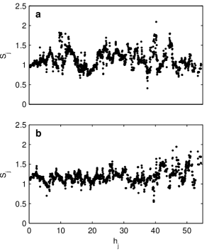
In Fig. 4 we plot of the residuals of ER Vul computed for three different values of the bins number . The empirical criteria for the computations of listed in Section 2.2 are satisfied for . But then the SC diagram is too smoothed even for (upper panel in Fig. 4) when the average number of per bin is 132. For this value reduces to 58, almost half of the bins contain less than 10 values and the SC diagram becomes irregular (lower panel in Fig. 4). Pop & Vamoş (2013) used the value for which the average number of per bin is 74 and only three bins at the end of the SC diagram contain less than 10 values.
The first minimum of located at yr is significantly higher than zero indicating a high noise level in the time series of ER Vul. We specify that thereafter, before the computation of the SC, every time series is always standardised, i.e. the average value is subtracted from it and then it is divided by its standard deviation.
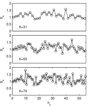
From the SC graphs displayed in Fig. 4 one can see that although in the first half of the SC exists one maximum and one minimum, their shape varies quite a lot as a function of . The minimum at yr is better defined for low values of , while when increases, a secondary local maximum appears in the region of this minimum. In the same way, for low values of the maximum situated at yr is well defined. On the contrary, when increases, another secondary maximum appears, sometimes even higher than the primary one. In fact, the maximum must occur at approximately yr, but as we can see in Fig. 2b (continuous line with circle markers), even for the simple sine function the first maximum is strongly distorted and shifted to the right due to the uneven sampling. These fluctuations could explain the less defined second minimum which should be located at yr.
In order to remove the shape fluctuations of , we apply the stacking method used in seismology, which enhances the deterministic signal when the seismograms are very noisy (Shearer, 2009). Instead of a single value of , we compute for several values, , and by superposing the corresponding SC values we obtain the ‘enhanced self-correlation’ (ESC). For each we obtain another grid , () on which we compute the corresponding SC values . We construct a thickened grid by putting together the bins centers of the grids for all . The new grid contains
values and we denote by , , its nodes arranged in ascending order and by the corresponding values of the SC. Figure 5a shows the ESC of the curve of ER Vul for and (). We chose the value according to the criteria given in the previous section. The value is chosen so that the ESC contains all the possible shapes of the extrema of individual SCs.
Using the ESC we can determine the interval of values which contains the most significant information concerning the deterministic component of the ER Vul time series. In the classical approach of the SC method there are no rigorous criteria for the choice of the optimum number of extrema to be used in the analysis (Percy et al., 2004). In the case of ER Vul, the shape of displayed in Fig. 5a confirms the existence of the two extrema identified in Fig. 4. They appear together with weakly defined additional extrema and we want to establish if they are the signature of the existence of a deterministic component. We compare their shape with those of in the case of Gaussian white noise having the ER Vul sampling (Fig. 5b). We see that in the first half the variations of for the Gaussian white noise have lower amplitude compared to that of ER Vul time series and display a random shape. In the second half of the two ESCs, both curves have fluctuations with higher amplitude than those appearing in the first half. Therefore, we have to find a suitable criteria in order to choose the region of ESC over which we perform the comparison.
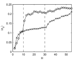
This separation of the properties of the ESC may be analysed through its variability on intervals , where is a given parameter. We denote by the standard deviation of the ESC over such an interval. We have computed , the average of over a statistical ensemble of 1000 Gaussian white noise, having the time sampling of the ER Vul data. The results are displayed in Fig. 6 together with for ER Vul time series. We can make the following remarks:
-
i.
For the variability of the ESC of ER Vul and that of Gaussian white noises are comparable. This means that the initial region of the ESC of ER Vul does not contain the signature of a deterministic component.
-
ii.
The difference between the variability of the two ESCs becomes significant for , i.e. in the region where the two main extrema of the ER Vul ESC are situated.
-
iii.
For , the variability of the ESC for Gaussian white noises increases much faster. In this region, the random fluctuations dominate both the ESC functions, and the difference between their variabilities diminishes.
4 Signal detection problem
Basically, the problem of the detection of a periodic signal in the presence of an additive noise is tackled through statistical tests [see e.g. Scargle (1982); Schwarzenberg-Czerny (1993, 1998, 2003); Kuschnig et al. (1997); Pop et al. (2010) (see also references therein), Appourchaux (2011)]. Usually, one claims the detection of a periodic signal if the power/amplitude of a suspected peak exceeds a level computed for a given threshold value of the probability of false alarm , i.e. the probability of the type I error that the observed time series is purely random. Alternatively, one may estimate the false alarm probability corresponding to the height of the considered spectral peak and compare it with a previously established threshold value , e.g. 0.1, 0.05, 0.03, 0.01, and 0.001 (Scargle, 1982; Black & Scargle, 1982; Horne & Baliunas, 1986; Kuschnig et al., 1997). Then, we may conclude that the observed time series consists not only of pure noise, but it contains a deterministic component. Moreover, due to the nature of the Fourier transform, from the amplitude/power spectrum analysis one may infer that the respective spectral peak is the signature of a periodic harmonic signal.
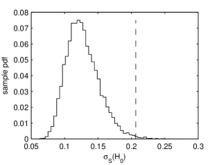
In the case of SC analysis we can design a statistical test for the existence of a deterministic component in the ER Vul time series, without any reference to its periodicity. The standard deviation of the ESC over the interval introduced in the previous section is an indicator for the existence of a deterministic component, not only for a periodic one. The difference of variability between the ESC of ER Vul and that of the Gaussian white noises occurs in the first half of ESC. Therefore, we choose as test statistic the standard deviation for yr.
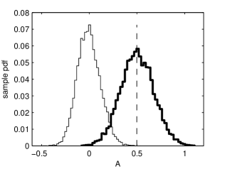
In Fig. 7 we display the sample pdf of obtained from a statistical ensemble of 10000 Gaussian white noises. We also marked the value of corresponding to the curve for ER Vul (dashed vertical line). In very few cases (0.5 per cent from all) the variability of the ESC for Gaussian white noise is greater than that observed for ER Vul. Then and we can reject the null hypothesis that the ER Vul time series is a Gaussian white noise at a confidence level of 99.5 per cent. This result does not significantly depend on the value of . For , the above confidence level takes values between 99.18 per cent and 99.74 per cent.
The false alarm probability value is one order of magnitude higher than that resulted from the Monte Carlo simulations relying on the amplitude spectrum performed by Pop & Vamoş (2013). When instead of the ESC method we have used the simple SC computed for a single value, we have obtained a value a few times larger. Although we have improved the result of the statistical test, however we have not reached the significance level of 0.001 which allows us to claim the detection of a deterministic signal in the residuals of ER Vul. The statistical test described above may be used indifferently of the shape of the deterministic component possibly existing in the analysed time series. If there is no indication that the deterministic component is periodic or at least quasi-periodic, then it has to be determined by a detrending algorithm. The resulting trend strongly depends on the noise level in the analysed time series (Vamoş & Crăciun, 2012).
5 Numerical model of ER Vul time series
We can further improve the detection of the deterministic component found in the residuals of ER Vul by introducing additional information concerning the periodicity of the detected signal. Pop & Vamoş (2013) proposed the following model for the cyclic variability of the curve of ER Vul
| (5) |
where , is the number of the analysed data, is the number of orbital cycles, and is a Gaussian white noise with zero mean and unit variance. The values of the model parameters were estimated via nonlinear least-squares method: d, , and rad. The final residuals obtained after removing the estimated periodic component have a standard deviation d.
This model was used by Pop & Vamoş (2013) to evaluate the detectability of the estimated periodic signal through Monte Carlo simulations. In order to approach this problem relying on the self-correlation method we have to take into account the effect emphasized by Welsh (1997). The presence of a Gaussian additive noise in the analysed time series determines an overestimation of the amplitude of a periodic harmonic signal existing in the data, either in the case of least-squares method, or in that of the amplitude spectrum computation. In the previous study of ER Vul the amplitude was computed by imposing the condition that the value of the highest peak in the spectrum of the observed data and in the averaged spectrum of a statistical ensemble of synthetic time series of the type (5) are equal (Pop & Vamoş, 2013). They obtained a lower value for the amplitude of the periodic component d.
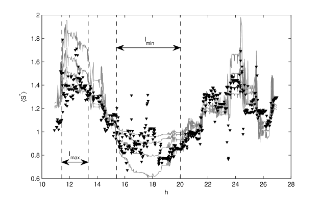
This time we impose the condition that the shapes of the ESC of the observational data and of the artificial time series are similar. We generate 100 artificial time series with a fixed value of the ratio . The numerical generation is performed in two steps. First, we use Eq. (5) with and and then we standardise it. For each artificial time series we compute the ESC for , the interval where we have established that the ESC of the observed data differ most from a Gaussian white noise (see Section 3 and Fig. 5). After that we compute the average over the statistical ensemble . We perform the same computation for several values of separated by a step .
In Figure 8 we display the averaged ESC for four values of the ratio . One notices that the difference between the extrema of ESCs decreases as the noise amplitude increases. The square norm of the difference between the ESC of the observed data and is a measure of the similarity of the two graphs. The minimum of this norm is obtained for . Taking into account that the ER Vul residuals are standardised using the standard deviation , it follows that the coefficients appearing in Eq. (5) are d and d.
6 The detectability of a noisy periodic signal
In Section 4 we have established only the existence of a deterministic component inside the ER Vul time series. Now we may use the numerical model presented in Section 5 for the estimation of the existence of a periodic signal, not only a deterministic one. We use the information related to the positions of the first two ESC extrema of the artificial time series with a periodic component to design a new statistical test. The position of these two extrema can be established from Fig. 8 in the regions where the differences between the ESC graphs for different values of are the largest. These regions have unequal widths due to the uneven sampling of the ER Vul data (in Fig. 2b the width of the first maximum is half of that of the first minimum).
Using this criterion we choose the interval yr which contains the values belonging to the first maximum of (the first two dashed vertical lines in Fig. 8). For the first minimum of we chose the interval yr (the last two dashed vertical lines in Fig. 8). We define the average peak-to-peak amplitude of ESC as the difference between the average of the ESC values belonging to the corresponding two intervals
| (6) |
where and are the number of values within the intervals and , respectively.
In the following we use the average amplitude of the ESC as a test statistic in order to evaluate the detectability of a periodic signal hidden in an additive noise. The statistical ensemble is composed of 10000 Gaussian white noises identical with those used in Section 4. The probability of false alarm is , i.e. one order of magnitude smaller than that obtained in Section 4 (Fig. 9). Hence the residuals of ER Vul analysed using the ESC method contain, with a very high confidence level (99.98 per cent), a deterministic component having a characteristic time scale of about 18 yr.
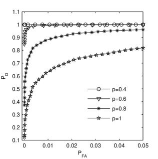
We have also generated statistical ensembles composed by 10000 artificial data sets relying on the model described by Eq. (5). The sample pdf of the average amplitude of the ESC for is plotted in Fig. 9. The value of the ‘observed’ mean amplitude of the ESC computed for the residuals of ER Vul allows the estimation of detectability of the inferred periodic signal [Scargle (1982); Schwarzenberg-Czerny (1998, 2003); Levy (2008); Sturrock & Scargle (2009); Appourchaux (2004, 2011); Johnson (2013); Pop & Vamoş (2013), see also references therein]. Assuming well-defined values of the parameters of the periodic model and for those describing the noise distribution, for a given ‘observed’ value of the considered statistic one can estimate the corresponding values of the probability of false alarm and of the probability of detection (or detection efficiency) . As it is well-known, these two quantities allow us to evaluate the detectability of the assumed periodic signal. The probability of detection represented as a function of the probability of false alarm is known as the ROC (Receiver Operating Characteristic) curve.
The ROC curves for the noise levels corresponding to those used in Fig. 8 are plotted in Fig. 10. The detectability of a periodic signal in ER Vul data depends strongly on the noise level and the chosen significance level. For the optimal model presented in Section 5 with , one remarks the following representative points on the run of the ROC curve (,): (0.001, 0.681), (0.01, 0.884), and (0.05, 0.960). For the ‘observed’ value of the average amplitude estimated from the ESC diagram one has and . Hence the high noise level in the data led to a low value of the detection probability, i.e. there is a high chance to obtain a non-detection result in the presence of the inferred signal. For lower noise levels the detection probability increases significantly, becoming almost ideal for (Fig. 10).
In the Bayesian approach we have the positive predicted value (the Bayesian detection rate)
and the negative predictive value
where and are the type I and the type II errors, respectively [see e.g. Levy (2008)]. According to Bayesian approach, the high indicates that the alternative hypothesis is very likely to be true, i.e. we have a very high chance to detect the inferred signal when it is really present in the analysed data. The relatively low indicates that, because of the high noise level in the data, there is a significantly high chance to obtain a detection result even when the inferred signal lacks from the data.
7 Conclusions
We have investigated the properties of the self-correlation function when it is used to search for periodicities in astronomical time series. We have considered the case of a harmonic periodic component existing in different types of time series with increasing complexity with respect to the sampling and to the presence of additive Gaussian white noise. We have begun with the ideal case of a continuous sinusoid defined on an infinite domain. In this case the minima of the SC function vanish and are situated at integer multiples of the period. The maxima occur at odd multiples of the half-period and are equal with , being the sinusoid amplitude. The second analysed case is that of a continuous sinusoid defined on a finite domain. The minima of the SC function are the same as in the previous case but the maxima are distorted, the distortion increasing with the time lag. The relation between the peak-to-peak amplitude of the SC function and that of the sinusoid remains approximately the same as above.
The following complication which we have introduced is the discretization of the finite continuous sinusoid. An equidistant grid does not distort the shape of the SC diagram, however, the level of minima of the SC does not vanish if the sampling interval of the time series is not a divisor of the period. For a non-equidistant grid (as the sampling of the ER Vul data) the positions of minima remain approximatively the same, but their levels become nonzero. The non-equidistant grid also induces large fluctuations in the region of maxima, so that their shapes can be determined only numerically. The proportionality between and is preserved, but its explicit form has to be also numerically studied.
Finally, we considered the case of realistic data by including in the last type of artificial time series the Gaussian white noise. We analytically derived the mathematical expression which allows us to estimate the standard deviation of the noise . The amplitude of the SC decreases when the noise level increases following a power law.
We have also investigated the statistical properties of the SC method especially concerning its ability to detect harmonic periodic signals hidden in noise and in unevenly sampled data. We propose an improvement of the SC method by applying ‘the stacking method’ used in seismology, which we call enhanced self-correlation (ESC) method. It achieves an enrichment of the statistics which allows us to obtain a better resolution of the SC diagram. Using ESC we have obtained through Monte Carlo simulations a value of the false alarm probability low enough to reject the null hypothesis that the residuals of ER Vul are only noise. The very low value of indicates that almost surely the observed time series plotted in Fig. 1 is not a Gaussian white noise. But the high level of the noise prevents the precise identification of the characteristics of its deterministic component. It could be a simple harmonic periodic signal or a multiple periodic one dominated by a single period or a quasiperiodic phenomenon.
For the evaluation of the detectability of the inferred deterministic component, we take into account the previous result of Pop & Vamoş (2013) which describes it by a periodic harmonic model, the involved periodicity being of about 18 yr. For this approach we considered a test statistic with a higher specificity with respect to the assumed model, i.e. the average peak-to-peak amplitude in the ESC estimated from the first two extrema. Taking into account the average peak-to-peak amplitude of the ESC estimated for the standardised ER Vul time series, and using the binary decision making formalism within both the frequentist and Bayesian approaches, we performed Monte Carlo simulations which led us to the quantities featuring the detectability of the assumed periodic modulation.
Our conclusion is that the presence of a periodic signal was correctly detected at very low values () and at very high values of (), but due to the high noise level in the observational data, there is also a high risk to get false detections (relatively low values of and ) when the periodic component lacks and the time series contains only noise. These results obtained through ESC method are in good agreement with those obtained by Pop & Vamoş (2013). The present methodology is complementary to that relying on the amplitude spectrum analysis, and supplies a further substantiation of the orbital period modulation of about 18 yr occurring in ER Vul. However, because of the unsatisfactory detectability of this periodicity, the new observational data on this eclipsing binary system have to be collected with great care in order to reduce as much as possible the level of the observational noise.
Acknowledgments
We thank the referee, Professor J.R. Percy, for useful comments.
References
- Appourchaux (2004) Appourchaux T., 2004, A&A, 428, 1039
- Appourchaux (2011) Appourchaux T., 2011, arXiv:1103.5352v2[astro-ph.IM]
- Black & Scargle (1982) Black D.C., Scargle J.D., 1982, ApJ, 263, 854
- Horne & Baliunas (1986) Horne J.H., Baliunas S.L., 1986, ApJ, 302, 757
- Johnson (2013) Johnson D.H., 2013, Statistical Signal Processing, http://www.ece.rice.edu/ dhj/courses/elec531/notes.pdf
- Kuschnig et al. (1997) Kuschnig R, Weiss W.W., Gruber R., Bely P.Y., Jenkner H., 1997, A&A, 328, 544
- Levy (2008) Levy B.C., 2008, Principles of Signal Detection and Parameter Estimation, Springer, New York
- Marinova & Percy (1999) Marinova M., Percy J. R., 1999, JAAVSO, 27, 122
- Percy (2007) Percy J. R., 2007, Understanding Variable Stars, Cambridge University Press, Cambridge, New York
- Percy & Long (2010) Percy J. R., Long J., 2010, JAAVSO, 38, 161
- Percy & Mohammed (2004) Percy J. R., Mohammed F., 2004, JAAVSO, 32, 9
- Percy & Palaniappan (2006) Percy J. R., Palaniappan R., 2006, JAAVSO, 35, 290
- Percy & Sen (1991) Percy J. R., Sen, L., 1991, IBVS, 3670
- Percy & Terziev (2011) Percy J. R., Terziev, E., 2011, JAAVSO, 39, 162
- Percy et al. (2003) Percy J. R., Hosik J., Leigh N. W. C., 2003, PASP, 115, 59
- Percy et al. (1981) Percy J. R., Jakate S. M., Matthews J. M., 1981, AJ, 86, 53
- Percy et al. (1993) Percy J. R., Ralli J. A., Sen L. V., 1993, PASP, 105, 287
- Percy et al. (2004) Percy J. R., Favaro E., Glasheen J., Ho B., 2004, ”Using Astrolab Selfcorrelation Software”, http://www.astro.utoronto.ca/percy/manual.pdf
- Percy et al. (2006a) Percy J. R., Gryc W. K., Wong J. C.-Y., Herbst W., 2006a, PASP, 118, 1390
- Percy et al. (2002) Percy J. R., Hosik J., Kincaide H., Pang C., 2002, PASP, 114, 551
- Percy et al. (2009) Percy J. R., Esteves S., Lin A., Menezes C., Wu S., 2009, JAAVSO, 37, 71
- Percy et al. (2006b) Percy J. R., Molak A., Lund H., Overbeek D., Wehlau A. F., Williams P. F., 2006b, PASP, 118, 805
- Percy et al. (2010) Percy J. R., Esteves S., Glasheen J., Lin A., Long J., Mashintsova M., Terziev E., Wu S., 2010, JAAVSO, 38, 151
- Pop (1996) Pop A., 1996, Romanian Astron. J., 6, 147
- Pop (1999) Pop A., 1999, IBVS, No. 4801
- Pop & Vamoş (2013) Pop A., Vamoş C., 2013, NewA, 23 – 24, 27
- Pop et al. (2010) Pop A., Vamoş C., Turcu V., 2010, AJ, 139, 425
- Scargle (1982) Scargle J.D., 1982, ApJ, 263, 835
- Schwarzenberg-Czerny (1993) Schwarzenberg-Czerny A., 1993, in Proc. of the ESO/ST-ECF Data Analysis Workshop, April 26-27, p. 149
- Schwarzenberg-Czerny (1998) Schwarzenberg-Czerny A., 1998, BaltA, 7, 43
- Schwarzenberg-Czerny (2003) Schwarzenberg-Czerny A., 2003, ASP Conf. Ser., 292,383
- Shearer (2009) Shearer P.M., 2009, Introduction to Seismology, 2nd Edition, Cambridge University Press, Cambridge.
- Sturrock & Scargle (2009) Sturrock, P.A., Scargle, J.D., 2009, ApJ, 706, 393.
- Vamoş & Crăciun (2012) Vamoş C., Crăciun M., 2012, Automatic trend estimation, Springer, Dordrecht.
- Welsh (1997) Welsh W.F, 1997, in Maoz D., Sternberg A., Leibowitz E.M. (Eds.), Astronomical Time Series, Astrophysics and Space Science Library, Kluwer Academic Publishers, Dordrecht, p. 171, vol. 218
Appendix A Self-correlation of a sinusoid
Equation (1) can be simplified when the definition domain of is infinite, for instance . Then the self-correlation is defined as the limit
If is periodic with period , then we choose with integer and the integral is the sum of equal integrals. Taking the limit , or , we obtain
| (7) |
Hence for an infinite periodic signal the integration interval is a period and does not depend on . In these conditions is periodic with the same period .
We compute the self-correlation for a sinusoid with , where the frequency is a real number and the period is . If the sinusoid is infinite, then applying Eq. (7) we obtain
| (8) |
The function has the period , but due to the absolute value in the expression of its period is , in accordance with the former theoretical reasoning. The maxima of are equal with and they occur for with integer, i.e. at half the distances between the minima of . In Fig. 2 the function is plotted with dashed line for and .
Now we consider the same sinusoid defined on the finite interval and Eq. (1) becomes
This integral is elementary, but due to the absolute value in the integrand we have to separate carefully the intervals over which the cosine has the same sign. We make the notations and , where is the integer part function. When , the cosine function in the integrand has several semiperiods with a constant sign in the integration interval. The inequality is satisfied only if and then . The integration result is given by Eq. (2).
Equation (2) has a simpler form if is integer
| (9) |
where we have introduced the index in order to emphasize that is integer. In this case the self-correlation function has a special property. For two different integers , there exists the function
| (10) |
which transforms the respective self-correlations
This transformation indicates that the graph of over the interval is obtained by squeezing the graph of .
We can also describe how the parts of these graphs are related between them. The function has equidistant zeros , and in each interval limited by them the graph of contains a hump. The function (10) transforms the zeros of into the last zeros of the function ()
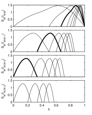
for every . In Fig. 11 we illustrate this transformation of the humps contained in the interval for different values of and fixed .
In the upper panel the last hump () is plotted, i.e. the graph of for . When , there is a single hump occupying the entire interval . For we have two humps and the last one is squeezed over the second half of the definition domain. For the last hump is even more compressed. In the second panel from the top the last but one humps () are plotted. Such humps exist only for . In this case the humps are translated and squeezed, but their values are not modified. A consequence of this transformation of the humps is that they have the same maximum value.
The graph of the function is composed by a succession of humps. For example, the graph with (the continuous line in Fig. 2) is composed by the three humps plotted with thick line in Fig. 11. Also the graph of can be obtained by compressing the graph of from the interval to and introducing the hump in the remained space. We recall that all these special properties hold only if is an integer.
In each interval there is a single maximum which can be obtained as an implicit solution of a trigonometric equation. If in Eq. (9) the integer part function is explicitly written, then for we have
where for and for . If we put the condition that the derivative of vanishes in the second part of the interval , we obtain for the position of the maximum in this interval the implicit formula
so we have
[1] Appourchaux T., 2004, A&A, 428, 1039
[2] Appourchaux T., 2011, in Pere L. P., Cesar E., eds, Asteroseismology. Cambridge Univ. Press, Cambridge, p. 123
[3] Black D. C., Scargle J. D., 1982, ApJ, 263, 854[4] Horne J. H., Baliunas S. L., 1986, ApJ, 302, 757[5] Johnson D. H., 2013, Statistical Signal Processing, http://www.ece.rice.edu/dhj/courses/elec531/notes.pdf
[6] Kuschnig R., Weiss W. W., Gruber R., Bely P. Y., Jenkner H., 1997, A&A, 328, 544
[7] Levy B. C., 2008, Principles of Signal Detection and Parameter Estimation. Springer-Verlag, Berlin
[8] Marinova M., Percy J. R., 1999, J. Am. Assoc. Var. Star Obs., 27, 122
[9] Percy J. R., 2007, Understanding Variable Stars. Cambridge Univ. Press, Cambridge
[10] Percy J. R., Long J., 2010, J. Am. Assoc. Var. Star Obs., 38, 161
[11] Percy J. R., Mohammed F., 2004, J. Am. Assoc. Var. Star Obs., 32, 9
[12] Percy J. R., Palaniappan R., 2006, 35, 290
[13] Percy J. R., Sen L., 1991, Inf. Bull. Var. Stars, 3670
[14] Percy J. R., Terziev E., 2011, J. Am. Assoc. Var. Star Obs., 39, 162
[15] Percy J. R., Jakate S. M., Matthews J. M., 1981, AJ, 86, 53
[16] Percy J. R., Ralli J. A., Sen L. V., 1993, PASP, 105, 287
[17] Percy J. R., Hosik J., Kincaide H., Pang C., 2002, PASP, 114, 551
[18] Percy J. R., Hosik J., Leigh N. W. C., 2003, PASP, 115, 59
[19] Percy J. R., Favaro E., Glasheen J., Ho B., 2004, Using Astrolab Selfcorrelation Software. http://www.astro.utoronto.ca/∼percy/manual.pdf
[20] Percy J. R., Molak A., Lund H., Overbeek D., Wehlau A. F., Williams P. F., 2006a, PASP, 118, 805
[21] Percy J. R., Gryc W. K., Wong J. C.-Y., Herbst W., 2006b, PASP, 118, 1390
[22] Percy J. R., Esteves S., Glasheen J., Lin A., Long J., Mashintsova M., Terziev E., Wu S., 2010, J. Am. Assoc. Var. Star Obs., 38, 151
[23] Pop A., 1996, Rom. Astron. J., 6, 147
[24] Pop A., 1999, Inf. Bull. Var. Stars, 4801, 1
[25] Pop A., Vamos¸ C., 2013, New Astron., 23–24, 27
[26] Pop A., Vamos¸ C., Turcu V., 2010, AJ, 139, 425 Scargle J. D., 1982, ApJ, 263, 835
[27] Schwarzenberg-Czerny A., 1993, in Grosbøl P. J., de Ruijsscher R. C. E., eds, Proc. of 5th ESO/ST-ECF, Data Analysis Workshop, No. 47, Garching b. Munchen: European Southern Observatory, p. 149 Schwarzenberg-Czerny A., 1998,
[28] Balt. Astron., 7, 43
[29] Schwarzenberg-Czerny A., 2003, in Sterken C., ed., ASP Conf. Ser. Vol. 292, Interplay of Periodic, Cyclic and Stochastic Variability in Selected Areas of the H-R Diagram. Astron. Soc. Pac., San Francisco, p. 383
[30] Shearer P. M., 2009, Introduction to Seismology, 2nd edn. Cambridge Univ. Press, Cambridge Sturrock P. A., Scargle J. D., 2009, ApJ, 706, 393
[31] Vamos¸ C., Craciun M., 2012, Automatic Trend Estimation. Springer-Verlag, Berlin
[32] Welsh W. F., 1997, in Maoz D., Sternberg A., Leibowitz E. M., eds, Astrophysics and Space Science Library, Vol. 218, Astronomical Time Series, Measuring Variability in the Presence of Noise. Kluwer, Dordrecht, p. 171
soon