
Abstract
In this paper, we introduce new max-product Shepard operators combined with Euler polynomial approximants, in both the univariate and bivariate cases. In each setting, we study the main approximation properties, including the degree of exactness and uniform error bounds. The bivariate construction of the Euler approximant is developed over a rectangle. Numerical experiments involving several test functions are performed to compare the approximation performance of the proposed operators with that of existing methods. Applications of the bivariate version of the operator are presented at the end of the paper. The applications consist of digital terrain reconstruction for several regions in Cluj County, Romania, and global approximation of precipitation quantities from 2025 and 2026.
Authors
Andra Malina
Faculty of Mathematics and Computer Science, Babeş-Bolyai University, Cluj-Napoca, Romania
Tiberiu Popoviciu Institute of Numerical Analysis, Romanian Academy, Cluj-Napoca, Romania
Keywords
max-product operator; Shepard operator; Euler polynomials; approximation error
Paper coordinates
A. Malina, Max-product Shepard-Euler operators, J. Comput. Appl. Math. 495 (2027), Art. No. 118327, https://doi.org/10.1016/j.cam.2026.118327
About this paper
Journal
Journal of Computational and Applied Mathematics
Publisher Name
Elsevier B.V.
Print ISSN
Online ISSN
1879-1778
Paper (preprint) in HTML form
Max-product Shepard-Euler operators
Abstract
In this paper, we introduce new max-product Shepard operators combined with Euler polynomial approximants, in both the univariate and bivariate cases. In each setting, we study the main approximation properties, including the degree of exactness and uniform error bounds. The bivariate construction of the Euler approximant is developed over a rectangle. Numerical experiments involving several test functions are performed to compare the approximation performance of the proposed operators with that of existing methods. Applications of the bivariate version of the operator are presented at the end of the paper. The applications consist of digital terrain reconstruction for several regions in Cluj County, Romania, and global approximation of precipitation quantities from 2025 and 2026.
keywords
max-product operator; Shepard operator; Euler polynomials; approximation error1 Introduction
The Shepard operator introduced in [29] is a powerful and widely used tool in approximating large scattered datasets, due to its easy generalization and small storage requirement. Considering a set of given nodes,
with available functional values for each , the operator is defined as
| (1) |
where denotes the Euclidean norm and is a control parameter.
The zero degree of exactness and the small accuracy in this form have led to the study of improved variants. These variants are obtained either by transforming the operator into a local one, thus improving its accuracy (see, e.g., [25]–[28]) or by using instead of the functional values , the values of another interpolation operator with higher degree of exactness. This approach has been studied in the univariate case, for example for the Shepard-Bernoulli variant [6], the Shepard-Abel-Goncharov operator [8], and the Shepard-Euler operator [31]. It has also been considered in the bivariate setting, including combinations with Lidstone operators [7, 9], Bernoulli-based combinations [10, 11, 17], and radial basis function approaches [12, 13]. More recently, related methods have been developed for spherical settings (see, for example, [2, 14, 15, 32, 33] and the references therein) due to the high applicability in practical problems, such as surface reconstruction, terrain modeling, image reconstruction, measurements for physical phenomena, solutions to partial differential equations and geophysical problems. Extensions to complex cases have also been studied (see, e.g., [18]).
One improvement of the univariate Shepard operator has been discussed in [31] and it regards the combination of the operator (1) with a generalized Taylor polynomial that uses the expansion in the Euler polynomials.
The Euler polynomials are defined as [5]
| (2) |
Lemma 1.1.
[31] The approximation formula for a function , with , and is
with the remainder term given by
| (4) |
where is the Peano kernel, i.e.,
| (5) |
Lemma 1.2.
Remark 1.3.
[31] We have that , with denoting the Taylor polynomial of degree around .
Remark 1.4.
Since , it follows that , for any .
Consider a set of given nodes in with and the fictive node . Wu defined the Shepard-Euler operator in [31] as
| (6) |
with and .
According to [31], the degree of exactness for this operator is .
Another class of Shepard-type operators is obtained by replacing the sum operator in (1) with the maximum operator, denoted by . Operators of this type were first introduced by Bede et al. in [3] and subsequently studied in [4]. To define the operator, let us consider the class of continuous nonnegative functions and some given sampling points. The max-product Shepard operator is given as [3]
| (7) |
with the maxitive Shepard kernel defined by
| (8) |
where denotes the Kronecker symbol
Remark 1.5.
The kernel functions satisfy the following property
| (9) |
Remark 1.6.
In contrast to the original Shepard interpolant, this operator is nonlinear. However, despite this drawback, operators of this type can provide better approximation properties when applied to nonnegative functions, as demonstrated in works such as [19], [22], and [23]. These studies focus on combinations of max-product Shepard operators with local interpolants based on Taylor, Bernoulli, and Lidstone polynomials. More generally, linear and nonlinear extensions of Shepard-type operators, together with accelerated convergence strategies and their applications are surveyed in [20]. In addition, the hybrid Shepard-Lagrange operators introduced in [21] provide a further example of improving the approximation properties of Shepard operators through the incorporation of local polynomial information.
Motivated by the fact that, as far as we are aware, the Shepard-Euler operator has been studied only in the linear univariate setting, we investigate its nonlinear version in the univariate case, develop its bivariate extension over a rectangle, and study its approximation properties, such as the degree of exactness and error estimates, in both settings. The paper is organized as follows. In Section 2, we study the max-product Shepard-Euler operator in the univariate case. In Section 3, we further examine this operator by providing numerical examples for several test functions. In Section 4, after extending the Euler approximant to the two-dimensional setting, we study the new bivariate Shepard operator obtained, and in Section 5, we investigate its practical behavior through numerical examples. Further, in Sections 6 and 7, we present two practical applications of the two-dimensional max-product Shepard-Euler operator. The first one consists of a digital terrain reconstruction problem of different regions from Cluj County, in Romania. The second one regards precipitation approximations around various regions of the globe in different months of 2025 and 2026. Section 8 concludes the paper.
2 The univariate max-product Shepard-Euler operator
In this section, we consider the class of nonnegative functions that have continuous -th order derivatives.
Definition 2.1.
Let and consider the given sample points , with the fictive node . We define the max-product Shepard-Euler operator of order as
| (10) |
with the kernel function given in (8), for any .
Proposition 2.2.
The operator given in (10) reproduces all nonnegative polynomials of degree at most .
Proof.
Theorem 2.3.
Let , consider the given sample points , with the fictive node , and . For the max-product Shepard-Euler operator given in (10), we have the following estimation of the error
| (11) |
where is the sup-norm, represents the integer part and is a constant depending on and .
Proof.
Let Using the result stated in (9) and [3, Lemma 3], we have that
Since represents the remainder term, denoted by , we have that
| (12) |
Let us define the distance from the interval as
| (13) |
From [22, Lemma 2], we have that
which gives us the following estimate
Denote by . We obtain
with .
- Case 1.
. We know from [22, Lemma 3] that Hence,
- Case 2.
. We have that on , so, for some such that . This implies that , so
If we choose and combine the two cases above, the conclusion follows.
∎
3 Numerical examples in the univariate case
To illustrate the approximation properties of the max-product Shepard–Euler operator introduced in (10), we consider the following test functions ), (see, e.g., [22]):
For each function we construct the max-product Shepard-Euler operator given in (10) by using sets of equidistant nodes in , for , and evaluate it on points in . We choose the parameters and . For a better visualization of the results, we compare the operator with the classical Shepard-Euler operator given in (6), the max-product Shepard operator defined in (7) and with the classical Shepard operator given in (1). The maximum approximation errors () and the mean approximation errors () are displayed in Table 1 for , in Table 2 for , and in Table 3 in the case of . It can be observed that the new operator introduced in this paper outperforms the other operators in the majority of the cases.
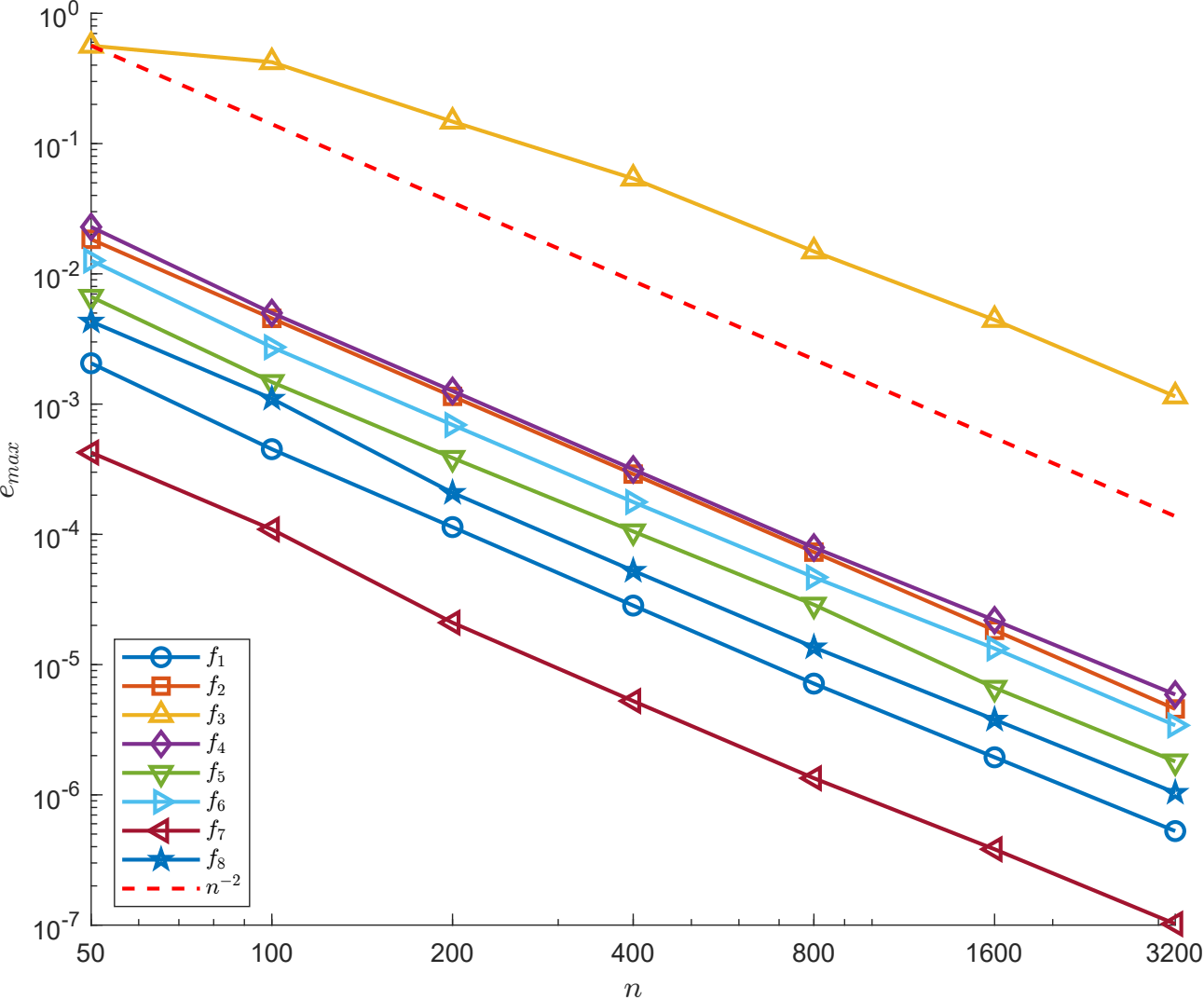
In what follows, we present in Figure 1 a log-log plot of the maximum error versus , for , , and the six test functions above, all of class . In addition, we also consider two functions that are only of class ,
For all eight functions, we consider , i.e., the operator such that the hypothesis of Theorem 2.3 is satisfied. As a reference, the red dotted line indicates a perfect quadratic trend. We can observe that the rate guaranteed by the theorem is obtained by all functions.
4 Bivariate max-product Shepard-Euler operator
Consider the rectangle and let be the space of functions that have continuous partial derivatives
for all with and .
For , and , we introduce the notations:
For , , we define the following functions:
with defined in (5) and
Using some ideas from [16], where the authors derive an expansion of a function over a rectangle in terms of Bernoulli polynomials, we obtain the following result.
Theorem 4.1.
For , , and , we have that
| (14) |
where
| (15) |
and
| (16) | ||||
Proof.
We follow some ideas presented in [16] to prove the result above. We first consider the particular case , , , so .
Using now the univariate expansion to each function of variable that appears in the right-hand side term, we obtain for each :
and
So, we get that:
| (17) |
with
and
To map the unit square to a rectangle defined by , , where and , we use the linear transformation [16]
Remark 4.2.
Similar to the univariate property stated in Remark 1.4, we have that , for any , with and .
Proposition 4.3.
Let be the space of polynomials of degree such that , . The operator given in (15) has the degree of exactness , i.e., , for any .
Proof.
Using the remainder formula given in (16), one can easily see that , for any ∎
The expansion obtained in Theorem 4.1 provides the local approximation tool that will subsequently be used in the definition of the bivariate max-product Shepard-Euler operator. In line with the strategy and ideas proposed in [30] for bivariate Bernoulli-type multiquadric quasi-interpolation operators, we next derive an explicit estimate for the corresponding local Euler remainder. This estimate will then be combined with the properties of the max-product Shepard kernel to obtain a uniform approximation bound for the global operator.
To study the remainder estimate even for points outside the rectangle , we consider the extended rectangle , with , (see, e.g., [30]). We first introduce the following notations from [31]. For , let
| (18) |
We consider the sup-norm of the function over its domain of definition, so, for , and for , .
Moreover, we introduce the general form of the distance given in (13), i.e., the distance of from the interval , plus , which is [31]
| (19) |
Theorem 4.4.
Proof.
Let . Here, we extend the definitions on of and to the rectangle , so, for and ,
with the kernels given by (5) and its analogue.
Using Lemma 5 to expand the representation of the remainder term from Theorem 4.1 to the rectangle , we have that , where
Based on the results stated in [31, Theorem 3] and the proof of [31, Theorem 2], it can be shown that for and ,
and, similarly, for and ,
Let us fix and set , for . Then, since and , we can observe that , i.e., exactly the univariate Euler operator given in (3) corresponding to the function on . By similar reasoning, for a fixed and , for , we obtain that .
Since , it follows that
Using analogous arguments, we have
Combining the relations above, we obtain
| (20) |
and, respectively,
| (21) |
For , straightforward computations show that
| (22) |
We now introduce the bivariate Euler-type max-product Shepard operator. To this end, for a rectangle , let denote the class of all functions such that , for any .
Definition 4.5.
Let and consider the sample points with , . For , we define the bivariate max-product Shepard-Euler operator of order as
| (23) |
where , , considering the fictive points , , and the kernel function given by
| (24) |
with denoting the Euclidean norm.
Proposition 4.6.
The operator given in (23) has the degree of exactness , i.e., , for any polynomial , where is the set of polynomials of degree such that , , and .
Proof.
The proof is similar to the one in the univariate case, since the degree of exactness of is (see Proposition 4.3) and the maxitive Shepard kernel satisfies the property ∎
Theorem 4.7.
Proof.
Let . Based on the property of the kernel and using similar reasoning as in the proof of Theorem 2.3, one can show that
| (25) |
At boundary nodes, where or , we reorder the endpoints independently in each affected coordinate. By the symmetry of the Euler polynomials (Remark 4.2), this leaves the local Euler approximant unchanged. Theorem 4.4 therefore applies with the ordered intervals and . The interval-distance terms in the subsequent estimates are understood with these ordered endpoints. Thus, by Theorem 4.4,
Let . Since and , from [22, Lemma 2] applied to each coordinate, we get that and . Moreover, since , we have that .
Combining these bounds, we get
where are defined as , , and .
Returning to (25) and letting denote the natural extension of the operator given in (7) to the bivariate case, we easily obtain that
We study the general term . As in the univariate case, we distinguish two cases:
Combining both cases, we obtain
Since is less than or equal to each of , we have that
Denoting , the conclusion follows. ∎
5 Numerical examples in the bivariate case
To validate the bivariate operator introduced in (23), we consider the following test functions ), (see, e.g., [19]):
For each function , , we construct the bivariate max-product Shepard-Euler operator defined in (23) over a uniform grid of nodes , . We choose and test the operators of degree and on two sets of sampling points, for and . The results are compared with those obtained using the classical bivariate Shepard-Euler operators and , as well as the bivariate max-product and classical Shepard operators, and , respectively. The first two types of operators are obtained by naturally extending, respectively, the univariate classical Shepard-Euler operator (6) and the univariate max-product Shepard operator (7) to the bivariate setting, while the classical Shepard operator is defined in (1). The maximum () and mean () approximation errors are presented in Tables 4 and 5.
It can be seen that the choice of higher approximation order significantly reduces the error with respect to . Moreover, increasing from to uniformly improves all operators, and, in this case, the max-product Shepard-Euler operator outperforms its classical version. Table 6 reports the CPU times for each operator across the four bivariate test functions, for . As expected, increasing the degree of the operator from to increases the runtime, since more terms of the Euler expansion must be evaluated at each node. Moreover, the computational cost of the classical and max-product versions of each operator are comparable, confirming that the max-product structure does not introduce significant overhead over its linear counterpart.
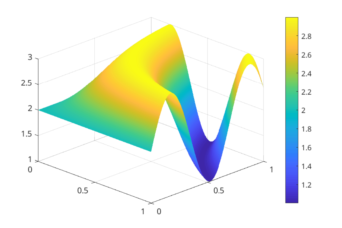
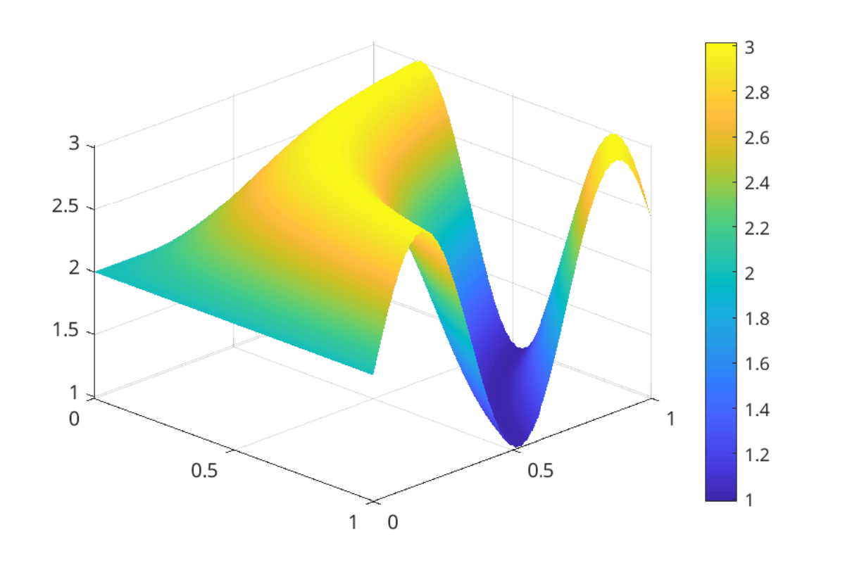
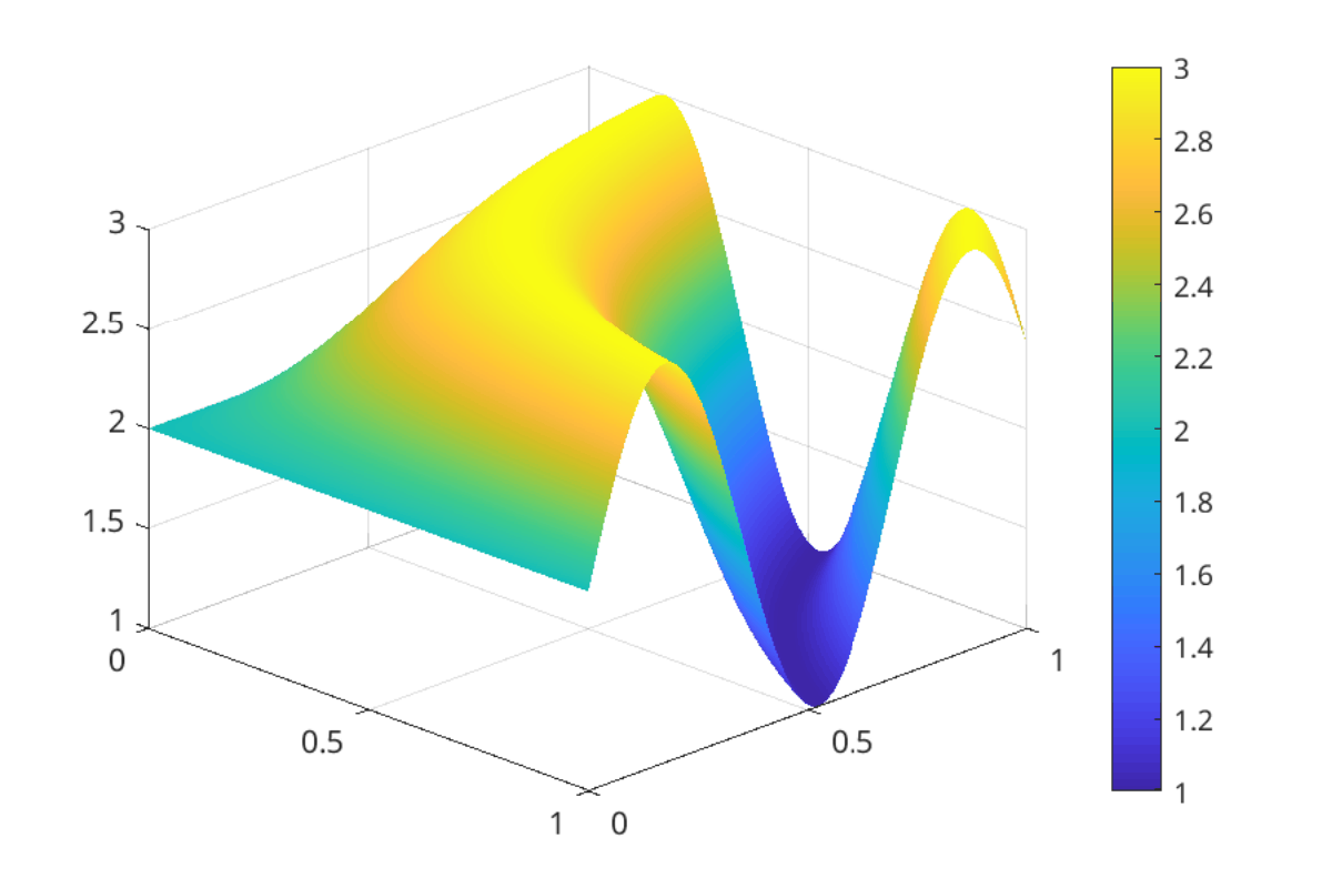
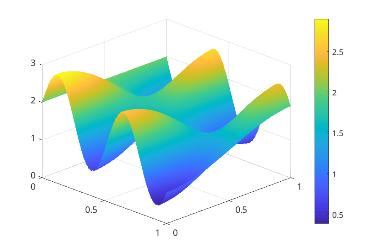
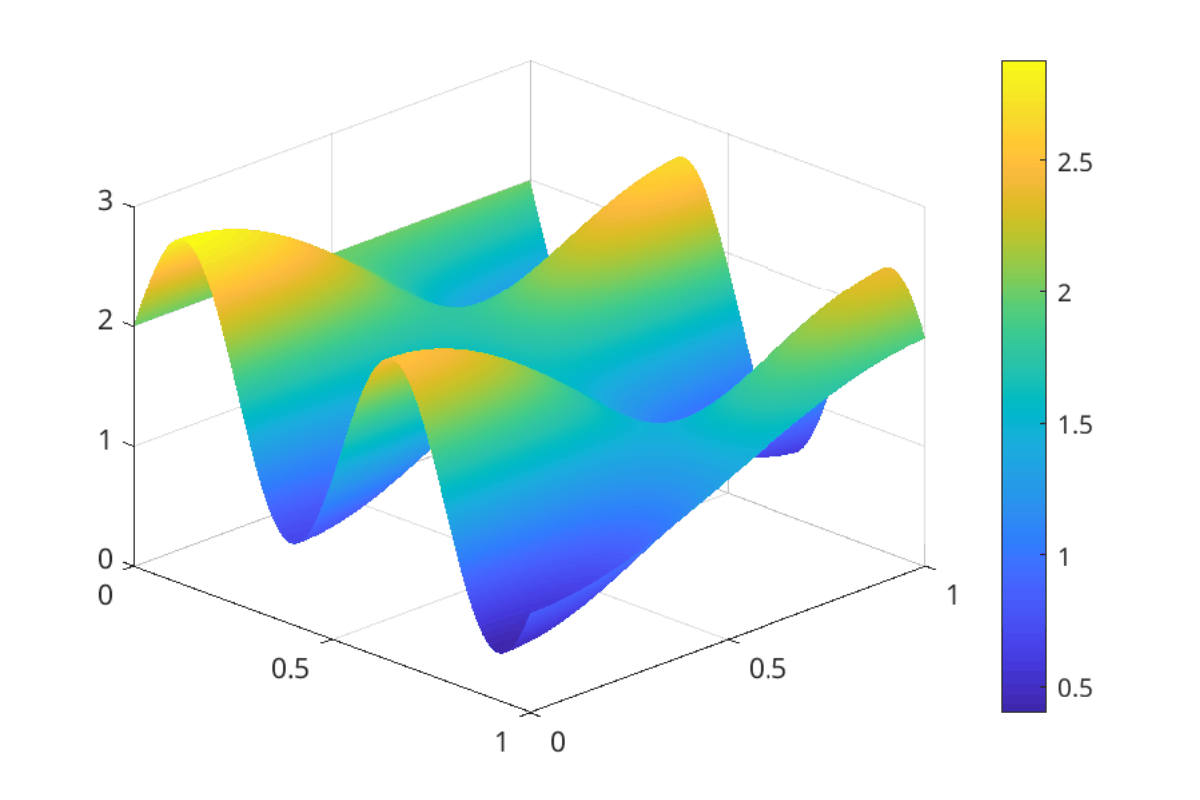
The graphical representations of the functions and the corresponding max-product Shepard-Euler approximants , , respectively, are displayed in Figures 2–4, in the case .
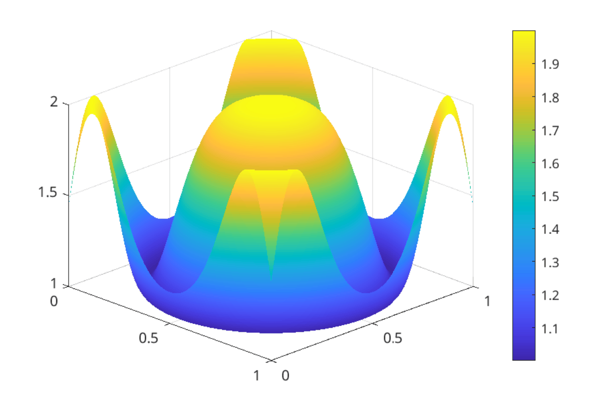
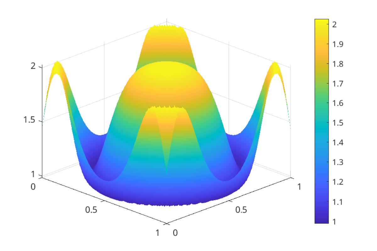
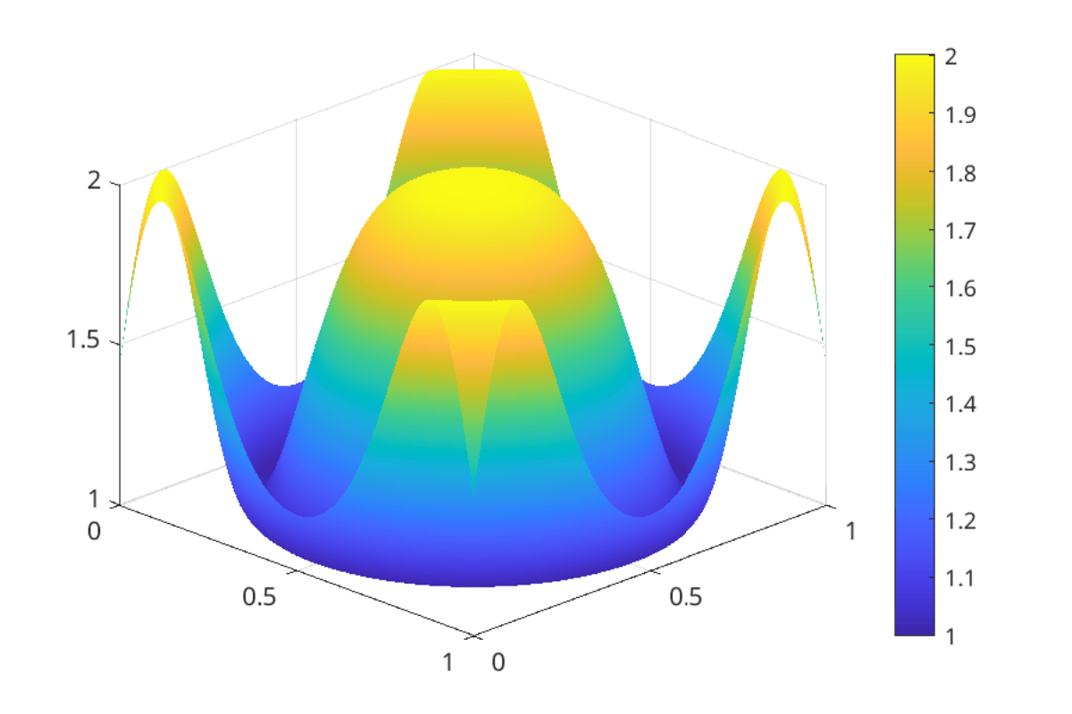
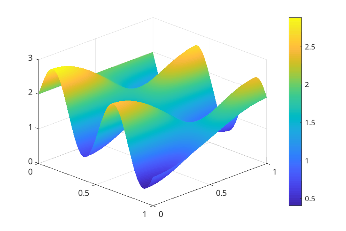
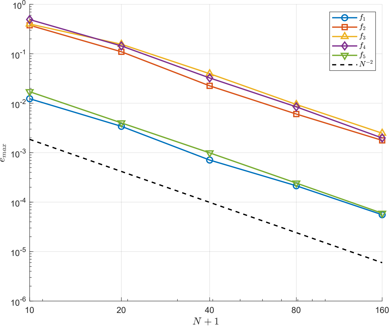
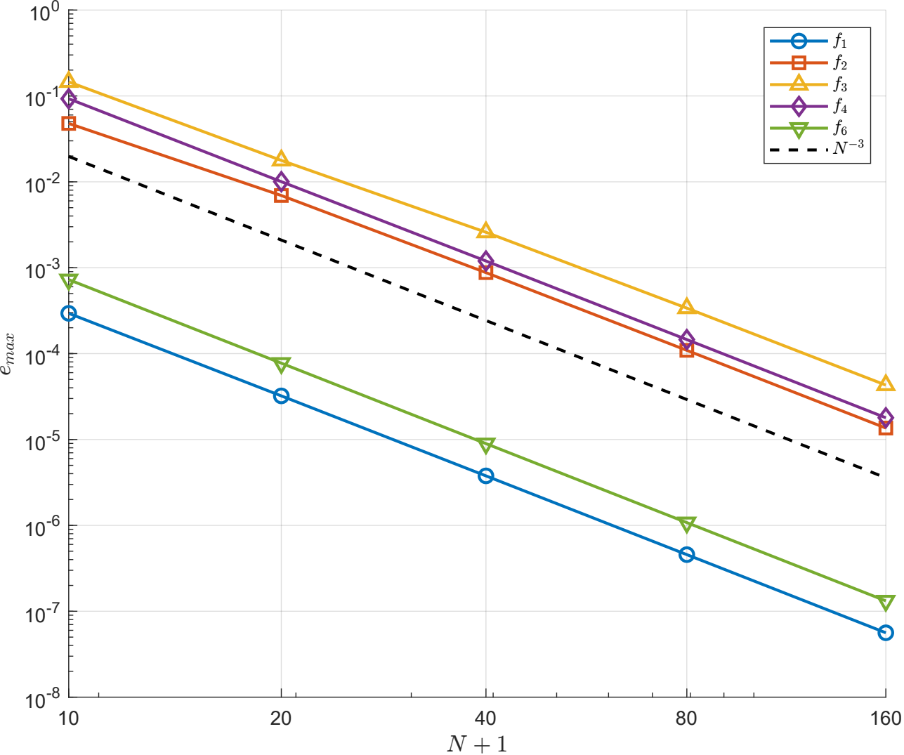
We next present, in Figure 5, log-log plots of the maximum error versus , for , . Subfigure 5(a) displays the results for the operator , applied to the four test functions introduced above (all of class ), and to a fifth function
which is only of class . For all five functions, the observed rates are close to (black dotted line), consistent with the rate guaranteed by Theorem 4.7. Subfigure 5(b) presents the analogous results for , applied to and to the function
only of class . Here, Theorem 4.7 guarantees an error bound of order at least , represented by the cubic trend given by the black dotted line.
Finally, to verify the degree of exactness, we test the operator on the polynomial functions
and display the mean approximation errors in Table 7. The results confirm Proposition 4.6: for , which is of degree , both and reproduce it to machine precision (errors of order ). For and , which are of degree , only reproduces them exactly (errors of order and , respectively). These results confirm that the degree of exactness of the operator is .
6 Application in a digital terrain reconstruction problem
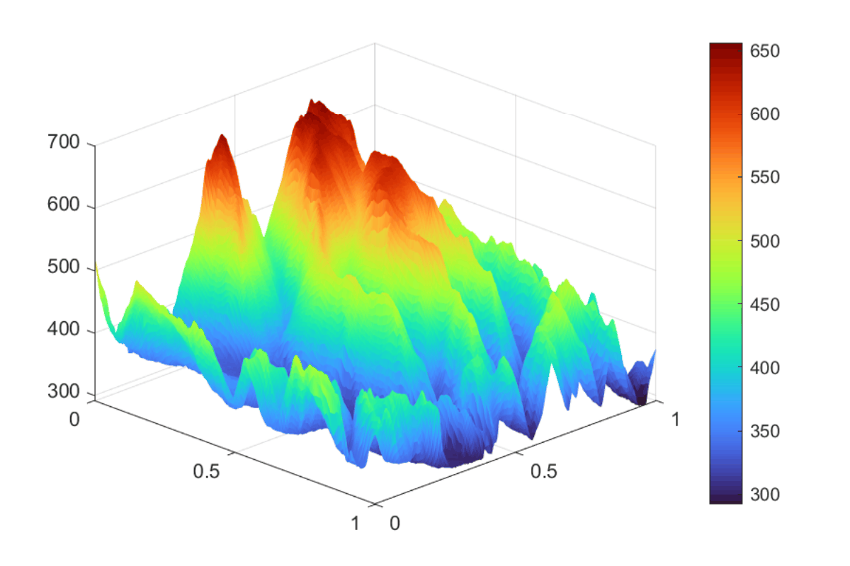
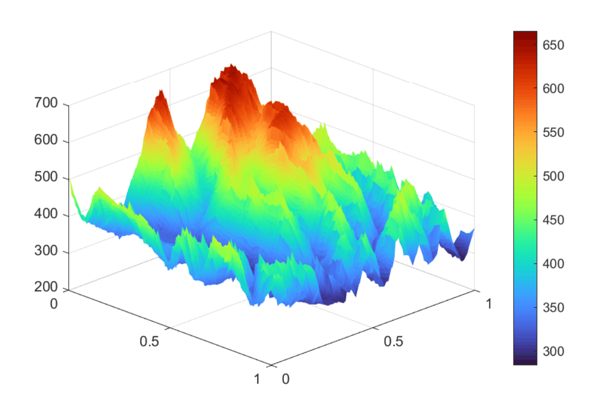
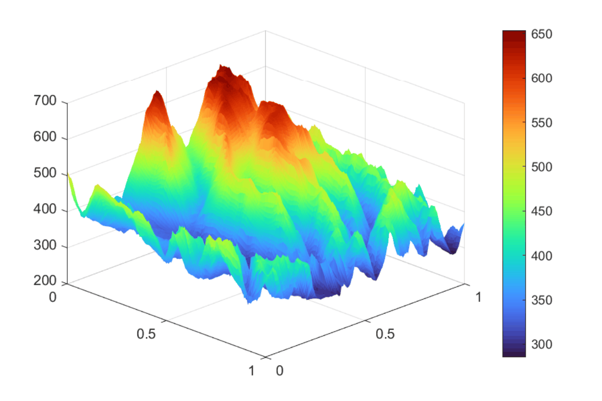
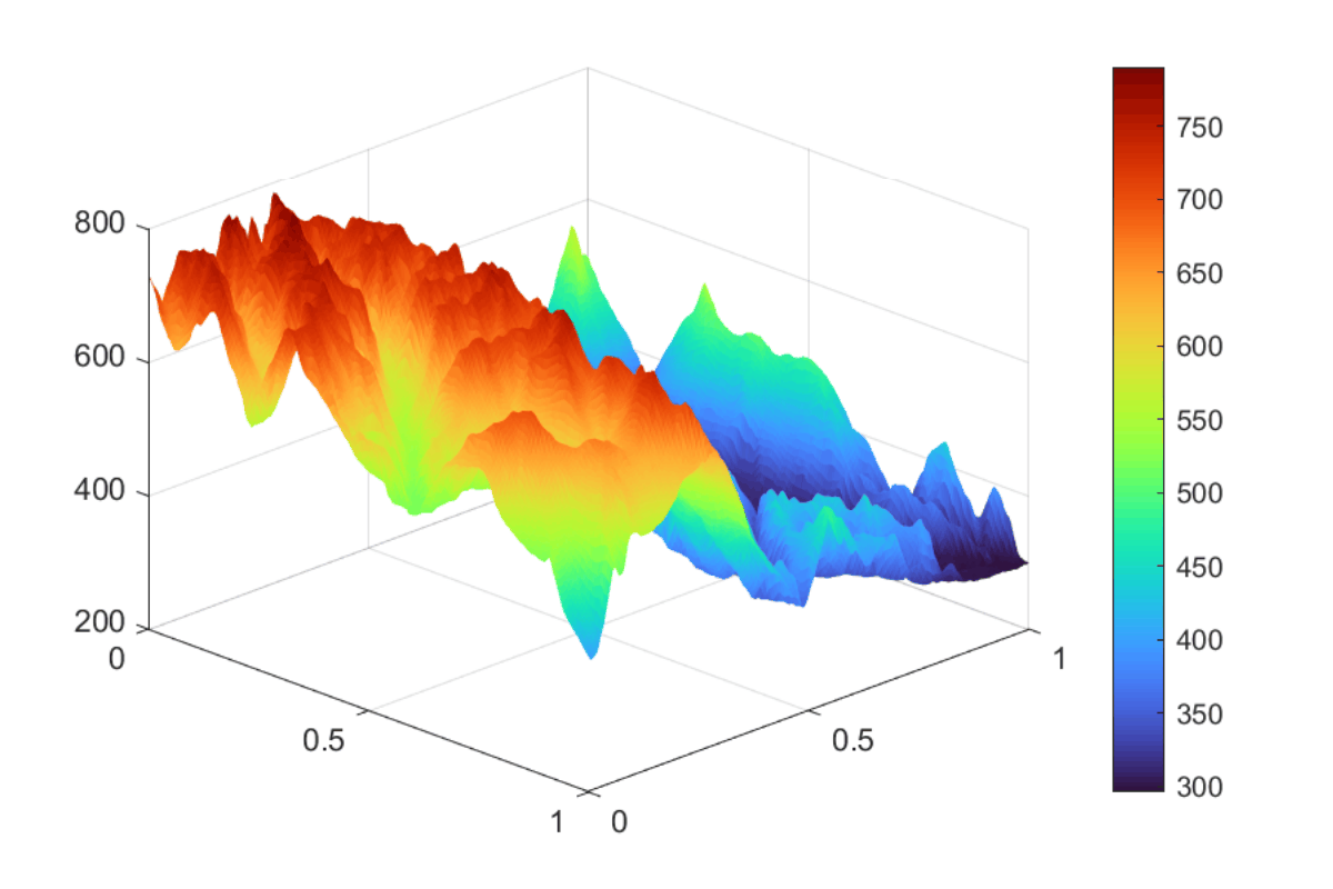
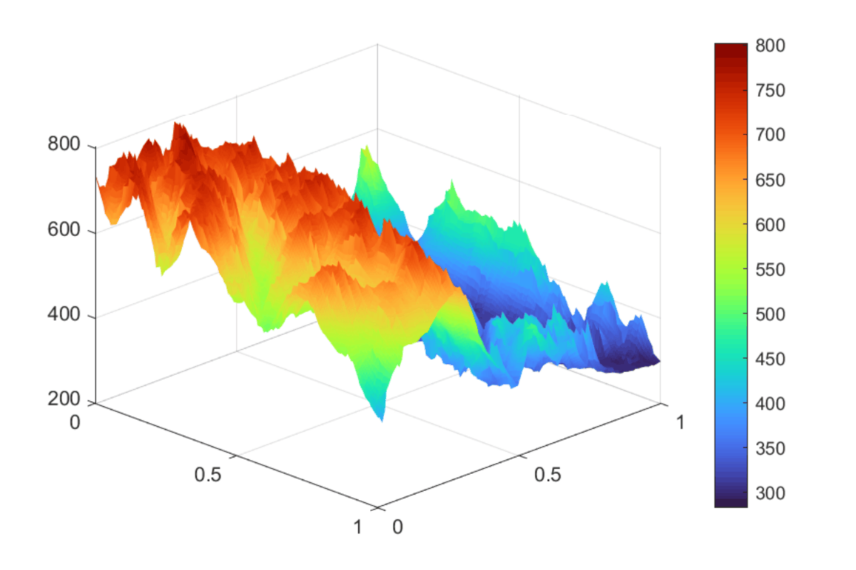
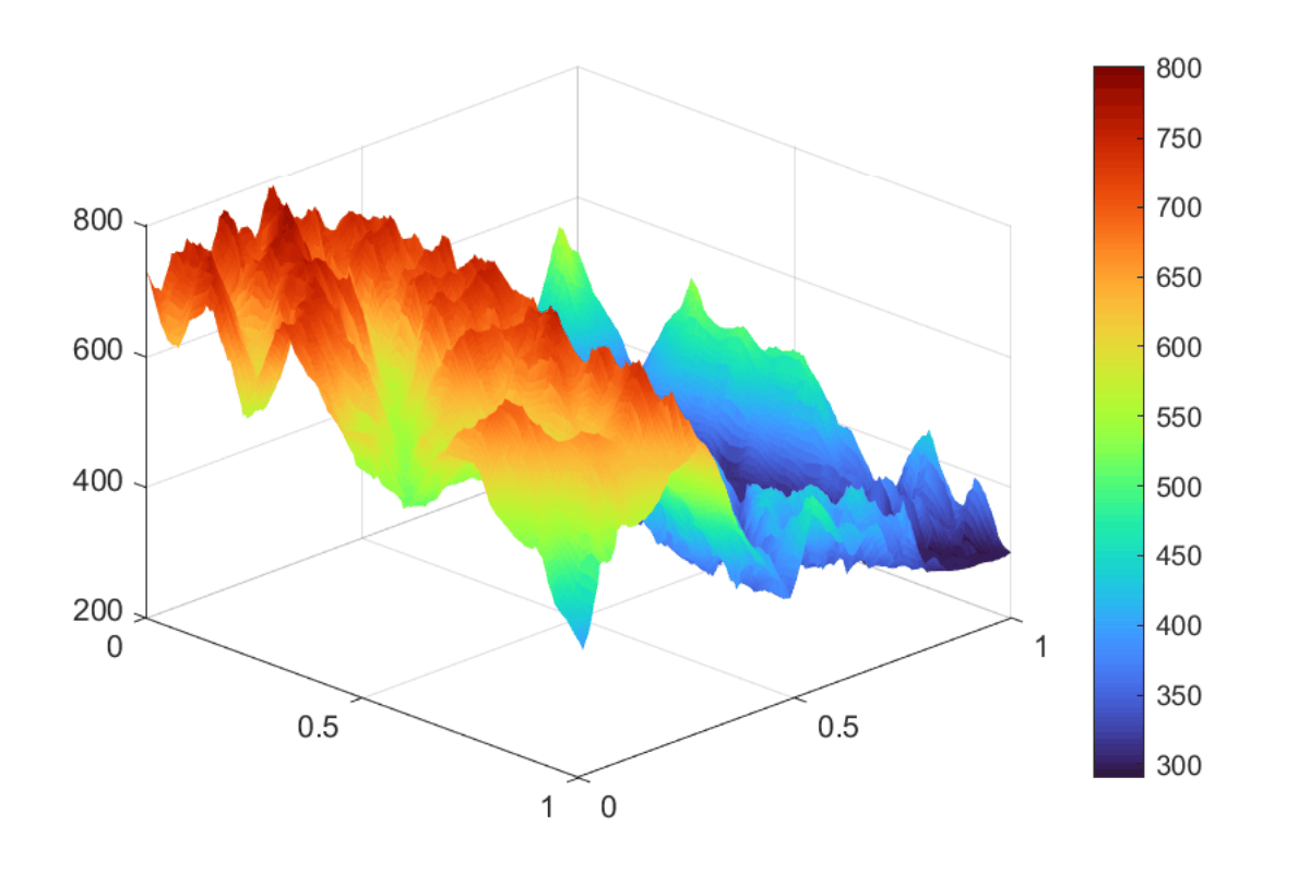
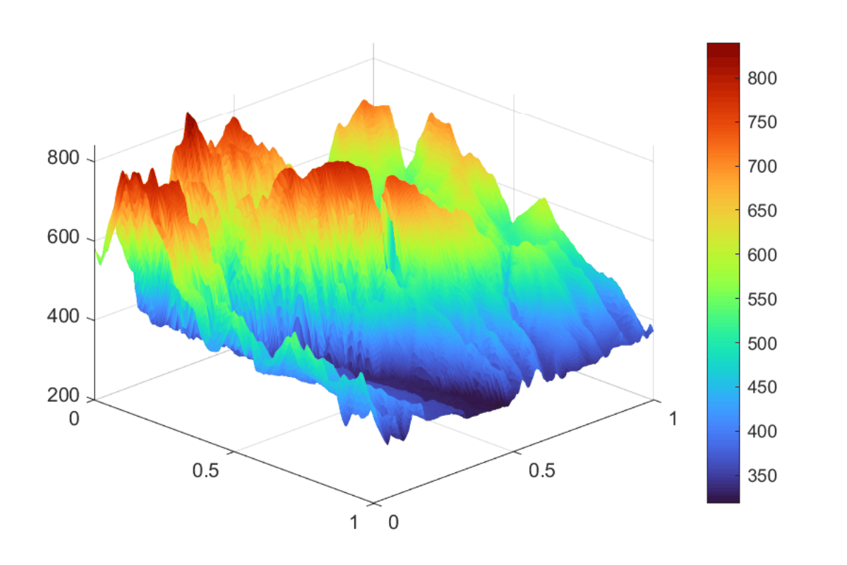
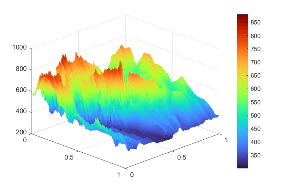
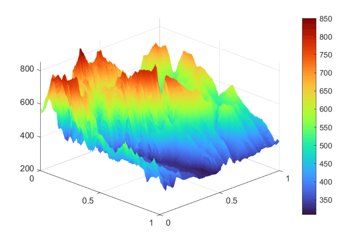
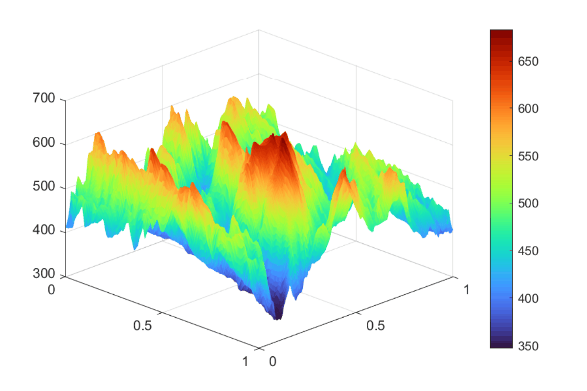
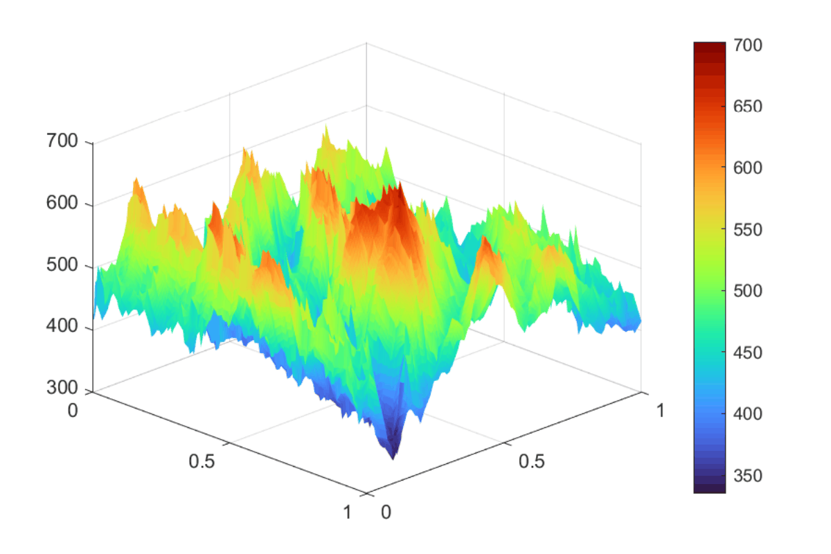
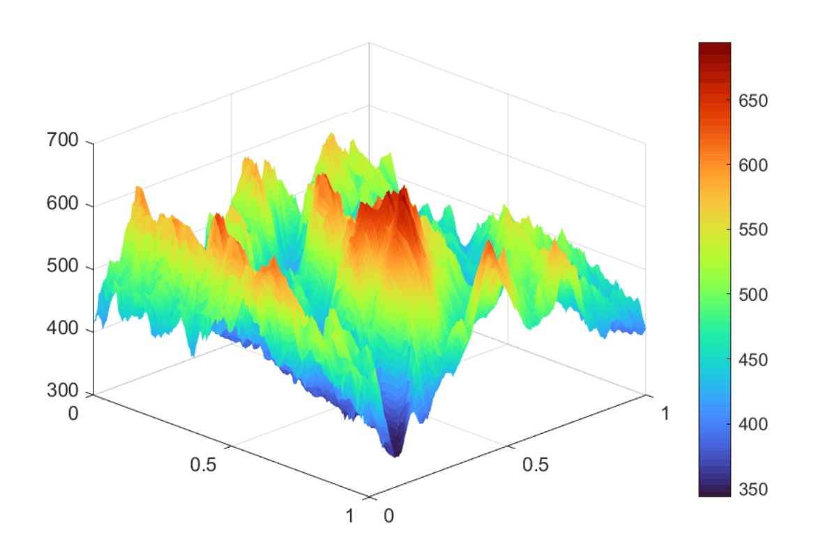
To evaluate the practical performance of the bivariate max-product Shepard–Euler operator introduced in this paper, we consider a digital terrain reconstruction problem across four different regions in Cluj County, in Romania. The data are extracted from the SRTM 1 Arc-Second Global dataset, tile N46E023 (N–N, E–E), provided by NASA and freely available via the NASA Earthdata portal at https://www.earthdata.nasa.gov/, or at https://download.mapsforge.org/maps/dem/dem3/N46/. We use two different sets of nodes, first considering , and then considering , and compute the approximation values on evaluation points.
The first dataset has altitudes between m and m. For the second dataset , the minimum value is m, and the maximum one is m. For dataset , the values are between m and m, while for the last one, , they are between m and m.
We apply the max-product Shepard-Euler operator given in (23), using MATLAB’s built-in gradient function to approximate the partial derivatives required in the construction of the operator. The substitution of exact partial derivatives with numerical estimates has also been considered in other interpolation studies. For example, Renka and Cline [27] proposed local derivative estimates obtained from quadratic weighted least-squares fits for a triangle-based interpolant. Dell’Accio and Di Tommaso [17] considered the case in which only function values are available and replaced derivative data by coefficients of locally fitted quadratic and cubic least-squares polynomials, obtaining comparable accuracy for the bivariate Shepard-Bernoulli operator. In our theoretical analysis from Section 4, however, the required partial derivatives are assumed to be known exactly, whereas in this application they are estimated from the available elevation data. Since SRTM-type elevation data are known to contain measurement errors, as mentioned in [24], the data approximations contain both operator and numerical differentiation errors. The latter cannot be assessed separately, since the exact terrain derivatives are unavailable. However, a more detailed investigation of the relation between numerical differentiation and data noise in this type of application represents a possible direction for future research.
To compare the results obtained, we also apply the classical Shepard-Euler operator , the max-product Shepard operator , and the classical Shepard operator on each dataset. The maximum and mean approximation errors are displayed in Table 8 for and in Table 9 for . It can be observed that combining the Shepard operator with the Euler polynomial approximant yields better results than the simple version of the Shepard operator, in both classical and max-product versions, in the majority of cases. Moreover, when using , the max-product Shepard-Euler operator has the smallest mean approximation errors across all datasets. The relative errors for this operator when applied to the dataset , are , when , and , when .
| m | m | m | m | m | m | m | m | |
| m | m | m | m | m | m | m | m | |
| m | m | m | m | m | m | m | m | |
| m | m | m | m | m | m | m | m | |
| m | m | m | m | m | m | m | m | |
| m | m | m | m | m | m | m | m | |
| m | m | m | m | m | m | m | m | |
| m | m | m | m | m | m | m | m | |
7 Application in precipitation quantities approximation
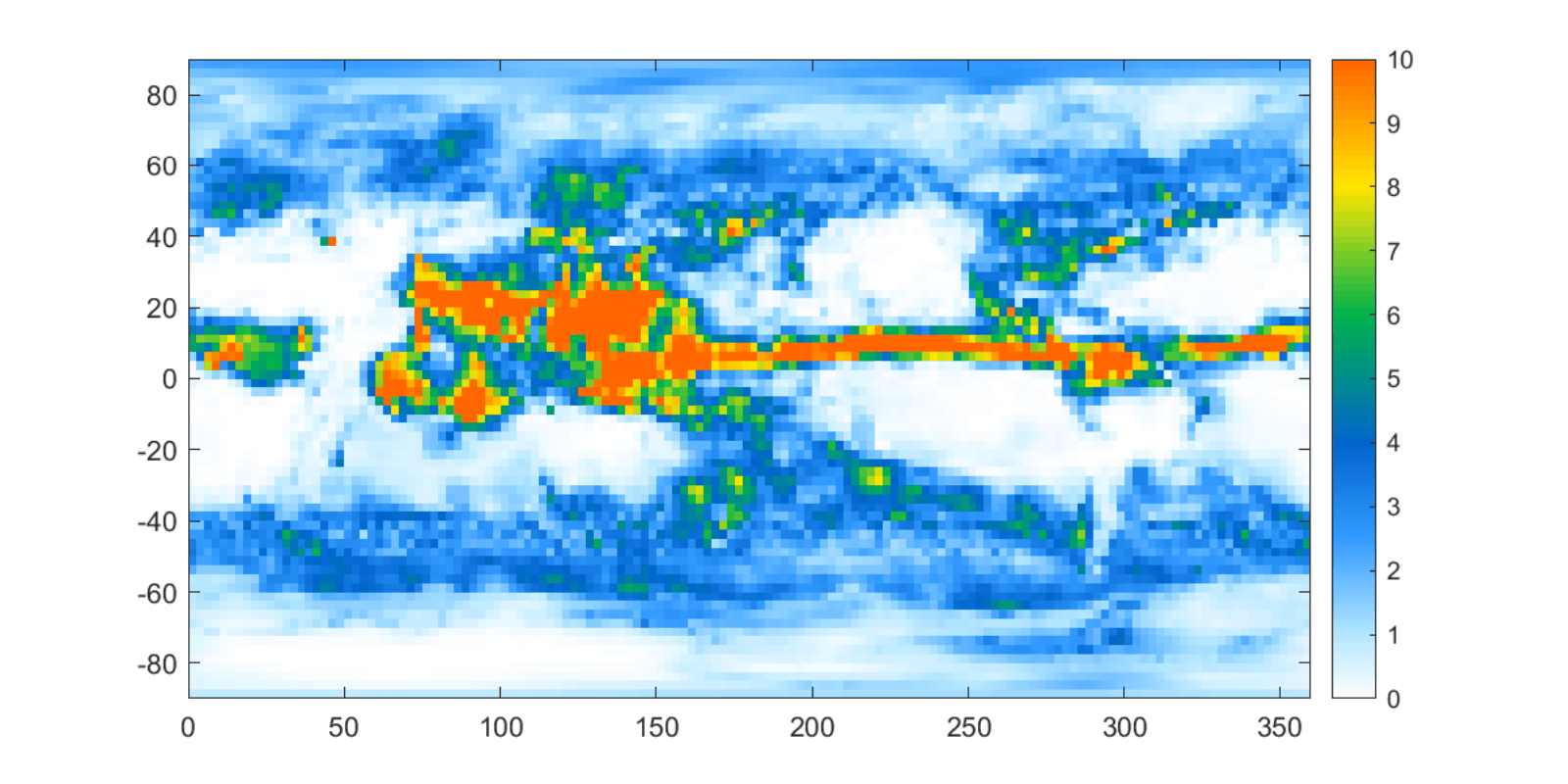
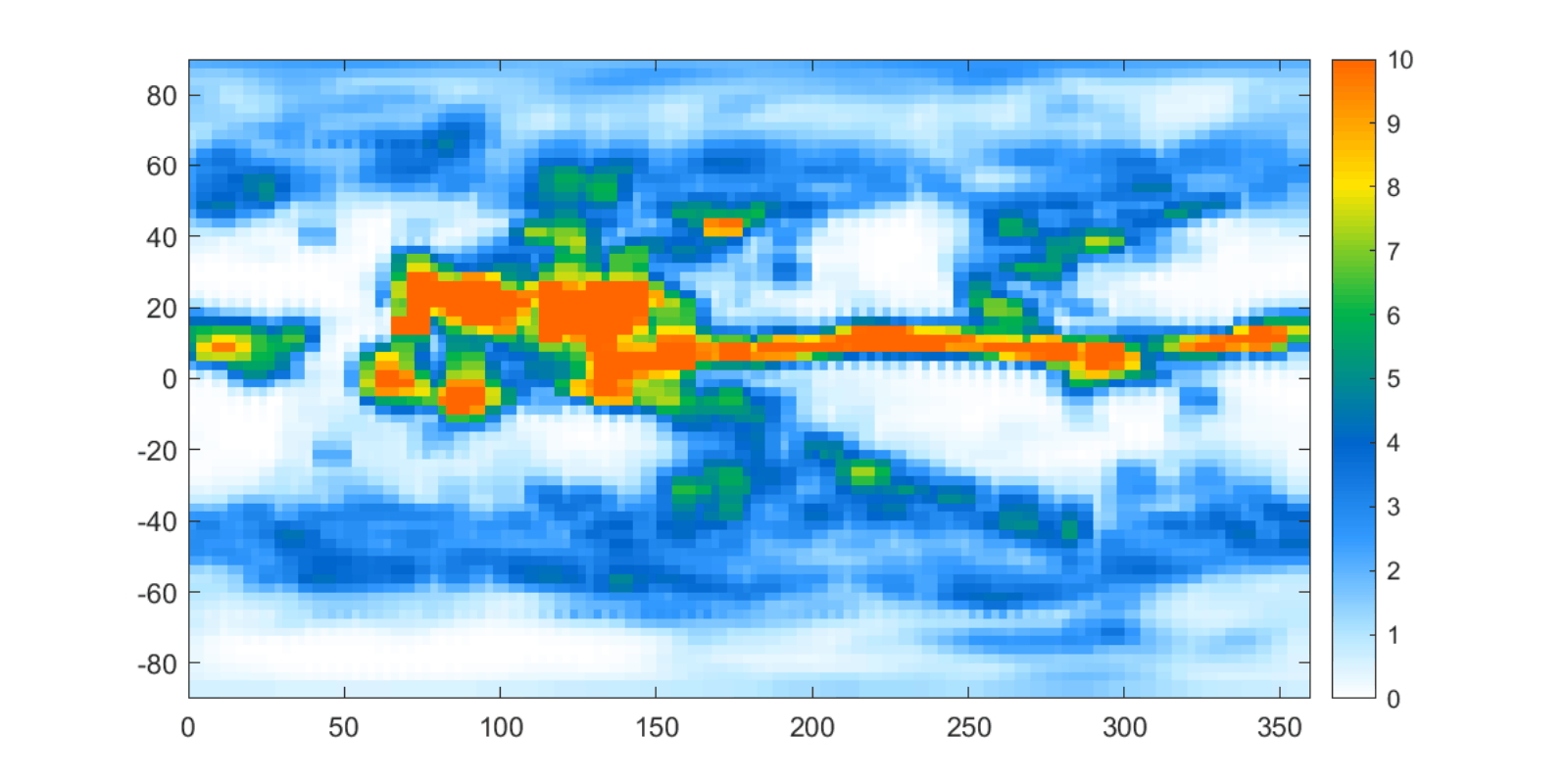
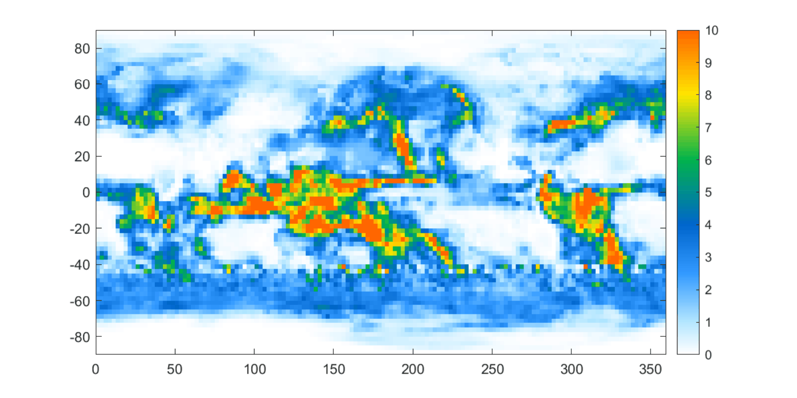
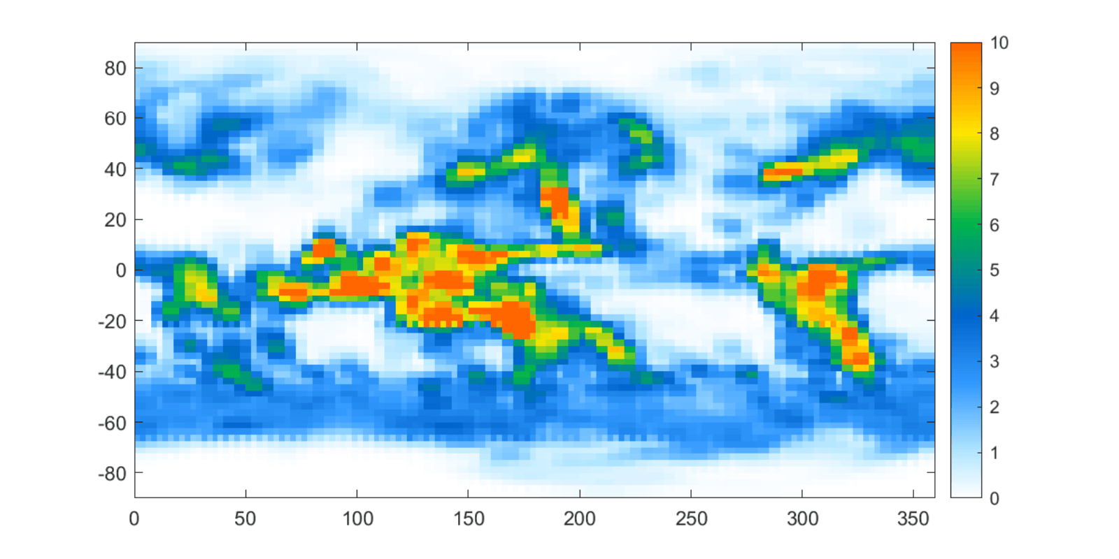
We end this paper by investigating another practical application of the bivariate operator introduced in this paper. We consider here the case to illustrate the operator’s behavior in this simplified setting which does not involve the partial derivatives of the function and compute the mean absolute errors in the approximation of some rainfall quantities over different months in and . The data set is available at https://psl.noaa.gov/data/gridded/data.gpcp.html and it is taken from the Global Precipitation Climatology Project (GPCP) Monthly Analysis product, distributed by the NOAA Physical Sciences Laboratory [1]. The dataset contains global monthly mean precipitation rates (mm/day) on a regular latitude–longitude global grid ( grid points) from January 1979 to present. We use nodes with to reconstruct values. The mean approximation errors () obtained with the bivariate max-product Shepard operator are displayed in Table 10. For each month, we display the minimum precipitation quantity () and the maximum one (). The graphical representations for the true and the approximated values in July 2025 and February 2026 are displayed in Figure 10 and Figure 11, respectively.
| 2025 | 2026 | |||||||
| Jan | Mar | May | Jul | Sep | Nov | Jan | Feb | |
| (mm/day) | ||||||||
| (mm/day) | ||||||||
| (mm/day) | ||||||||
8 Conclusion
In this paper, we introduced a novel max-product Shepard-type operator. The main contribution is the combination of the max-product Shepard framework with a local approximation operator based on Euler polynomials, with the aim of improving the performance of the classical Shepard operator for the approximation of nonnegative functions. We studied the approximation errors and the degree of exactness in both the univariate and bivariate settings. In addition to numerical examples involving several test functions, we considered practical applications, including terrain reconstruction and the approximation of precipitation data. Future work may address extensions to higher-dimensional settings and alternative local approximants.
Acknowledgments
The author would like to thank the anonymous referees for their careful reading of the manuscript and for their helpful suggestions, which have substantially improved this work.
References
- [1] Adler, R.F., Huffman, G.J., Chang, A., Ferraro, R., Xie, P., Janowiak, J., Rudolf, B., Schneider, U., Curtis, S., Bolvin, D., Gruber, A., Susskind, J., Arkin, P.: The Version 2 Global Precipitation Climatology Project (GPCP) Monthly Precipitation Analysis (1979-Present). J. Hydrometeor. 4, 1147–1167 (2003)
- [2] Allasia, G., Cavoretto, R., De Rossi, A.: Hermite-Birkhoff interpolation on scattered data on the sphere and other manifolds. Appl. Math. Comput. 318, 35–50 (2018)
- [3] Bede, B., Nobuhara, H., Fodor, J., Hirota, K.: Max-Product Shepard approximation operators. J. Adv. Comput. Intell. Intell. Inform. 10(4), 494–497 (2006)
- [4] Bede, B., Nobuhara, H., Daňková, M., Di Nola, A.: Approximation by pseudo-linear operators. Fuzzy Sets Syst. 159(7), 804–820 (2008)
- [5] Bretti, G., Ricci, P. E.: Euler polynomials and the related quadrature rule. Georgian Math. J. 8(3), 447–453 (2001)
- [6] Caira, R., Dell’Accio, F.: Shepard-Bernoulli operators. Math. Comp. 76, 299–321 (2007)
- [7] Caira, R., Dell’Accio, F., Di Tommaso, F.: On the bivariate Shepard–Lidstone operators. J. Comput. Appl. Math. 236, 1691–1707 (2012)
- [8] Cătinaş, T.: The combined Shepard-Abel-Goncharov univariate operator. J. Numer. Anal. Approx. Theory 32, 11–20 (2003)
- [9] Cătinaş, T.: The combined Shepard-Lidstone bivariate operator. In: Trends and Applications in Constructive Approximation. International Series of Numerical Mathematics (de Bruin, M.G. et al. (eds.)), 151, 77–89, Springer Group-Birkhäuser Verlag (2005)
- [10] Cătinaş, T.: The bivariate Shepard operator of Bernoulli type. Calcolo 44, 189–202 (2007)
- [11] Cătinaş, T.: An iterative modification of Shepard–Bernoulli operator. Results Math. 69, 387-395 (2016)
- [12] Cătinaş, T., Malina, A.: Shepard operator of least squares thin-plate spline type. Stud. Univ. Babeş-Bolyai Math. 66(2), 257–265 (2021)
- [13] Cătinaş, T., Malina, A.: The combined Shepard operator of inverse quadratic and inverse multiquadric type. Stud. Univ. Babeş-Bolyai Math. 67, 579–589 (2022)
- [14] Cătinaş, T., Malina, A.: Spherical interpolation of scattered data using least squares thin-plate spline and inverse multiquadric functions. Numer. Algor. 97, 1397–1414 (2024)
- [15] Cătinaş, T., Malina, A.: Spherical Shepard-Bernoulli operator. J. Appl. Math. Comput. 71, 1267–1283 (2025)
- [16] Costabile, F.A., Dell’Accio, F.: Expansion over a rectangle of real functions in Bernoulli polynomials and applications. BIT 41, 451–464 (2001)
- [17] Dell’Accio, F., Di Tommaso, F.: Bivariate Shepard–Bernoulli operators. Math. Comput. Simulation 141, 65–82 (2017)
- [18] Duman, O., Della Vecchia, B.: Complex Shepard operators and their summability. Results Math. 76, Art. No. 214 (2021)
- [19] Duman, O.: Max-product Shepard operators based on multivariable Taylor polynomials. J. Comput. Appl. Math. 437, Art. No. 115456 (2024)
- [20] Duman, O.: Shepard operators revisited: Linear and nonlinear approaches, accelerated convergence, and applications. Approx. Theory Spec. Funct. 1(1), 93–105 (2025)
- [21] Duman, O.: Improved approximation via hybrid Shepard–Lagrange operators: Linear and nonlinear perspectives. J. Comput. Appl. Math. 473, Art. No. 116864 (2026)
- [22] Ellidokuz, T. Y. G.: Approximation with max-product Shepard-Bernoulli operators. J. Comput. Appl. Math. 482, Art. No. 117313 (2026)
- [23] Ellidokuz, T. Y. G.: Approximation with Shepard-Lidstone and max-product Shepard-Lidstone operators. J. Comput. Appl. Math. 489, Art. No. 117922 (2027)
- [24] Falorni, G., Teles, V., Vivoni, E. R., Bras, R. L., Amaratunga, K. S.: Analysis and characterization of the vertical accuracy of digital elevation models from the Shuttle Radar Topography Mission. J. Geophys. Res. 110, Art. No. F02005 (2005)
- [25] Franke, R.: Scattered data interpolation: tests of some methods. Math. Comp. 38, 181–200 (1982)
- [26] Franke, R., Nielson, G.: Smooth interpolation of large sets of scattered data. Int. J. Numer. Meths. Engrg. 15, 1691–1704 (1980)
- [27] Renka, R.J., Cline, A.K.: A triangle-based interpolation method. Rocky Mountain J. Math. 14, 223–237 (1984)
- [28] Renka, R.J.: Multivariate interpolation of large sets of scattered data. ACM Trans. Math. Software 14, 139–148 (1988)
- [29] Shepard, D.: A two dimensional interpolation function for irregularly spaced data. In: Proceedings of the 1968 23rd ACM National Conference, 517–523. ACM (1968)
- [30] Wu, R.: A kind of bivariate Bernoulli-type multiquadric quasi-interpolation operator with higher approximation order. J. Inequal. Appl. 2023, Art. No. 88 (2023)
- [31] Wu, R.: A kind of univariate improved Shepard-Euler operators. Open Mathematics 23(1), Art. No. 20250209 (2025)
- [32] Zerroudi, B., Tayeq, H., El Harrak, A.: Effective interpolation of scattered data on a sphere through a Shepard-like method. Math. Model. Comput., 10(4), 1174–1186 (2023)
- [33] Zerroudi, B., Tayeq, H., El Harrak, A.: Scattered data interpolation on the 2-dimensional surface through Shepard-like technique. Math. Model. Comput. 11(1), 277–289 (2024)
[1] D. Shepard, A two dimensional interpolation function for irregularly spaced data, in: Proceedings of the 1968 23rd ACM National Conference, ACM, 1968, pp. 517–523.
[2] R. Franke, Scattered data interpolation: tests of some methods, Math. Comp. 38 (1982) 181–200.
[3] R. Franke, G. Nielson, Smooth interpolation of large sets of scattered data, Int. J. Numer. Meths. Engrg. 15 (1980) 1691–1704.
[4] R.J. Renka, A.K. Cline, A triangle-based 1 interpolation method, Rocky Mountain J. Math. 14 (1984) 223–237.
[5] R.J. Renka, Multivariate interpolation of large sets of scattered data, ACM Trans. Math. Software 14 (1988) 139–148.
[6] R. Caira, F. Dell’Accio, Shepard-Bernoulli operators, Math. Comp. 76 (2007) 299–321.
[7] T. Cătinaș, The combined Shepard-Abel-Goncharov univariate operator, J. Numer. Anal. Approx. Theory 32 (2003) 11–20.
[8] R. Wu, A kind of univariate improved Shepard-Euler operators, Open Math. 23 (1) (2025) Art. No 20250209.
[9] R. Caira, F. Dell’Accio, F. Di Tommaso, On the bivariate Shepard-Lidstone operators, J. Comput. Appl. Math. 236 (2012) 1691–1707.
[10] T. Cătinaș, The combined Shepard-Lidstone bivariate operator, in: M.G. de Bruin et al., (Eds.), Trends and Applications in Constructive Approximation, 151 of International Series of Numerical Mathematics, Springer Group-Birkhäuser Verlag, 2005, pp. 77–89.
[11] T. Cătinaș, The bivariate Shepard operator of Bernoulli type, Calcolo 44 2007 189–202.
[12] T. Cătinaș, An iterative modification of Shepard-Bernoulli operator, Results Math. 69 (2016) 387–395.
[13] F. Dell’Accio, F. Di Tommaso, Bivariate Shepard-Bernoulli operators, Math. Comput. Simulation 141 (2017) 65–82.
[14] T. Cătinaș, A. Malina, Shepard operator of least squares thin-plate spline type, Stud. Univ. Babeș-Bolyai Math. 66 (2) (2021) 257–265.
[15] T. Cătinaș, A. Malina, The combined Shepard operator of inverse quadratic and inverse multiquadric type, Stud. Univ. Babeș-Bolyai Math. 67 (2022) 579–589.
[16] G. Allasia, R. Cavoretto, A. De Rossi, Hermite-Birkhoff interpolation on scattered data on the sphere and other manifolds, Appl. Math. Comput. 318 (2018) 35–50.
[17] T. Cătinaș, A. Malina, Spherical interpolation of scattered data using least squares thin-plate spline and inverse multiquadric functions, Numer. Algor. 97 (2024) 1397–1414.
[18] T. Cătinaș, A. Malina, Spherical Shepard-Bernoulli operator, J. Appl. Math. Comput. 71 (2025) 1267–1283.
[19] B. Zerroudi, H. Tayeq, A. El Harrak, Effective interpolation of scattered data on a sphere through a Shepard-like method, Math. Model. Comput. 10 (4) (2023) 1174–1186.
[20] B. Zerroudi, H. Tayeq, A. El Harrak, Scattered data interpolation on the 2-dimensional surface through Shepard-like technique, Math. Model. Comput. 11 (1) (2024) 277–289.
[21] O. Duman, B. Della Vecchia, Complex Shepard operators and their summability, Results Math. 76 () (2021).
[22] G. Bretti, P.E. Ricci, Euler polynomials and the related quadrature rule, Georgian Math. J. 8 (3) (2001) 447–453.
[23] B. Bede, H. Nobuhara, J. Fodor, K. Hirota, Max-Product Shepard approximation operators, J. Adv. Comput. Intell. Intell. Inform. 10 (4) (2006) 494–497.
[24] B. Bede, H. Nobuhara, M. Danková, A. Di Nola, Approximation by pseudo-linear operators, Fuzzy Sets Syst. 159 (7) (2008) 804–820.
[25] O. Duman, Max-product Shepard operators based on multivariable Taylor polynomials, J. Comput. Appl. Math. 437, (2024), Art. No.115456
[26] T.Y.G. Ellidokuz, Approximation with max-product Shepard-Bernoulli operators, J. Comput. Appl. Math. 482 (2026).
[27] T.Y.G. Ellidokuz, Approximation with Shepard-Lidstone and max-product Shepard-Lidstone operators, J. Comput. Appl. Math. 489 (2027).
[28] O. Duman, Shepard operators revisited: linear and nonlinear approaches, accelerated convergence, and applications, Approx. Theory Spec. Funct. 1 (1) (2025) 93–105.
[29] O. Duman, Improved approximation via hybrid Shepard–Lagrange operators: linear and nonlinear perspectives, J. Comput. Appl. Math. 473 (2026)
[30] F.A. Costabile, F. Dell’Accio, Expansion over a rectangle of real functions in Bernoulli polynomials and applications, BIT 41 (2001) 451–464.
[31] R. Wu, A kind of bivariate Bernoulli-type multiquadric quasi-interpolation operator with higher approximation order, J. Inequal. Appl. 2023 (2023).
[32] G. Falorni, V. Teles, E.R. Vivoni, R.L. Bras, K.S. Amaratunga, Analysis and characterization of the vertical accuracy of digital elevation models from the Shuttle Radar Topography Mission, J. Geophys. Res. 110 (2005) Art. No. F02005.
[33] R.F. Adler, G.J. Huffman, A. Chang, R. Ferraro, P. Xie, J. Janowiak, B. Rudolf, U. Schneider, S. Curtis, D. Bolvin, A. Gruber, J. Susskind, P. Arkin, The Version 2 Global Precipitation Climatology Project (GPCP) Monthly Precipitation Analysis (1979-Present), J. Hydrometeor. 4 (2003) 1147–1167.