Shepard operator of least squares thin-plate spline type

2 years ago

approximation of multivariate functions, Approximation Theory, not-at-ICTP, Shepard

Abstract

We obtain some new Shepard type operators based on the classical, the modified Shepard methods and the least squares thin plate spline function. Given some sets of points, we compute some representative subsets of knot points following an algorithm described by J. R. McMahon in 1986.

Authors

Teodora Catinas
Babes-Bolyai University, Faculty of Mathematics and Computer Sciences

Andra Malina

Babes-Bolyai University, Faculty of Mathematics and Computer Sciences

Tiberiu Popoviciu Institute of Numerical Analysis, Romanian Academy

Keywords

Scattered data; Shepard operator; least squares approximation; thinplate spline; knot points.

Paper coordinates

Malina Andra, Catinas Teodora, Shepard operator of least squares thin-plate spline type, Stud. Univ. Babes-Bolyai Math. 66(2021), No. 2, 257–265
http://doi.org/10.24193/subbmath.2021.2.02

PDF

http://www.cs.ubbcluj.ro/~studia-m/index.php/journal/article/view/1242/pdf

About this paper

Journal

Studia

Publisher Name

Univ. Babes-Bolyai Math.

DOI

10.1016/0309-1708(91)90002-6

Print ISSN

0252-1938

Online ISSN

2065-961X

MR

ZBL

Google Scholar

https://scholar.google.com/citations?user=_yNNgu4AAAAJ&hl=ro

Paper (preprint) in HTML form

Shepard operator of least squares thin-plate spline type

Teodora Cătinaş “Babeş-Bolyai” University,
Faculty of Mathematics and Computer Sciences
1, Kogălniceanu Street,
400084 Cluj-Napoca,
Romania tcatinas@math.ubbcluj.ro Andra Malina “Babeş-Bolyai” University,
Faculty of Mathematics and Computer Sciences
1, Kogălniceanu Street,
400084 Cluj-Napoca,
Romania andra.malina@stud.ubbcluj.ro

Abstract.

Key words and phrases:

Scattered data, Shepard operator, least squares approximation, thin plate spline, knot points.

1991 Mathematics Subject Classification:

41A05, 41A25, 41A80.

1. Preliminaries

One of the best suited methods for approximating large sets of data is the Shepard method, introduced in 1968 in [16]. It has the advantages of a small storage requirement and an easy generalization to additional independent variables, but it suffers from no good reproduction quality, low accuracy and a high computational cost relative to some alternative methods [15], these being the reasons for finding new methods that improve it (see, e.g.,[1]-[8], [17], [18]). In this paper we obtain some new operators based on the classical, the modified Shepard methods and the least squares thin plate spline.

Let $f$ be a real-valued function defined on $X\subset\mathbb{R}^{2},$ and $(x_{i},y_{i})\in X,\;\\ i=1,...,N$ some distinct points. Denote by $r_{i}\left(x,y\right)$ the distances between a given point $\left(x,y\right)\in X$ and the points $\left(x_{i},y_{i}\right),\;i=1,...,N$ . The bivariate Shepard operator is defined by

\left(S_{\mu}f\right)\left(x,y\right)={\sum\limits_{i=1}^{N}}A_{i,\mu}\left(x,% y\right)f\left(x_{i},y_{i}\right),

(1.1)

where

A_{i,\mu}\left(x,y\right)=\frac{{\textstyle\prod\limits_{\begin{subarray}{c}j=% 1\\ j\neq i\end{subarray}}^{N}}r_{j}^{\mu}\left(x,y\right)}{{\textstyle\sum\limits% _{k=1}^{N}}{\textstyle\prod\limits_{\begin{subarray}{c}j=1\\ j\neq k\end{subarray}}^{N}}r_{j}^{\mu}\left(x,y\right)},

(1.2)

with the parameter $\mu>0.$

It is known that the bivariate Shepard operator $S_{\mu}$ reproduces only the constants and that the function $S_{\mu}f$ has flat spots in the neighborhood of all data points.

Franke and Nielson introduced in [10] a method for improving the accuracy in reproducing a surface with the bivariate Shepard approximation. This method has been further improved in [9], [14], [15], and it is given by:

\left(Sf\right)\left(x,y\right)=\frac{{{\textstyle\sum\limits_{i=1}^{N}}}W_{i}% \left(x,y\right)f\left(x_{i},y_{i}\right)}{{{\textstyle\sum\limits_{i=1}^{N}}}% W_{i}\left(x,y\right)},

(1.3)

with

W_{i}\left(x,y\right)=\left[\tfrac{(R_{w}-r_{i})_{+}}{R_{w}r_{i}}\right]^{2},

(1.4)

where $R_{w}$ is a radius of influence about the node $(x_{i},y_{i})$ and it is varying with $i .$ $R_{w}$ is taken as the distance from node $i$ to the $j$ th closest node to $(x_{i},y_{i})$ for $j>N_{w}$ ( $N_{w}$ is a fixed value) and $j$ as small as possible within the constraint that the $j$ th closest node is significantly more distant than the $(j-1)$ st closest node (see, e.g. [15]). As it is mentioned in [11], this modified Shepard method is one of the most powerful software tools for the multivariate approximation of large scattered data sets.

2. The Shepard operators of least squares thin-plate spline type

Consider $f$ a real-valued function defined on $X\subset\mathbb{R}^{2},$ and $(x_{i},y_{i})\in X,\;\\ i=1,...,N$ some distinct points. We introduce the Shepard operator based on the least squares thin-plate spline in four ways.

Method 1.

We consider

(S_{1}f)(x,y)={\sum\limits_{i=1}^{N}}A_{i,\mu}(x,y)F_{i}(x,y),

(2.1)

where $A_{i,\mu},$ $i=1,...,N,$ are defined by (1.2), for a given parameter $\mu>0$ and the least squares thin-plate splines are given by

F_{i}(x,y)={\textstyle\sum\limits_{j=1}^{i}}C_{j}d_{j}^{2}\log(d_{j})+ax+by+c,% \ \ i=1,...,N,

(2.2)

with $d_{j}=\sqrt{(x-x_{j})^{2}+(y-y_{j})^{2}}.$

For the second way, we consider a smaller set of $k\in\mathbb{N}^{*}$ knot points $(\hat{x}_{j},\hat{y}_{j}),$ $j=1,...,k$ that will be representative for the original set. This set is obtained following the next steps (see, e.g., [12] and [13]):

Algorithm 2.1.

1.

Generate $k$ random knot points, with $k<N$ ;
2.

Assign to each point the closest knot point;
3.

If there exist knot points for which there is no point assigned, move the knot to the closest point;
4.

Compute the next set of knot points as the arithmetic mean of all corresponding points;
5.

Repeat steps 2-4 until the knot points do not change for two successive iterations.

Method 2.

For a given $k\in\mathbb{N}^{*}$ , we consider the representative set of knot points $(\hat{x}_{j},\hat{y}_{j}),$ $j=1,...,k$ . The Shepard operator of least squares thin-plate spline is given by

(S_{2}f)(x,y)={\sum\limits_{i=1}^{k}}A_{i,\mu}(x,y)F_{i}(x,y),

(2.3)

where $A_{i,\mu},$ $i=1,...,k,$ are defined by

A_{i,\mu}\left(x,y\right)=\frac{{\textstyle\prod\limits_{\begin{subarray}{c}j=% 1\\ j\neq i\end{subarray}}^{k}}r_{j}^{\mu}\left(x,y\right)}{{\textstyle\sum\limits% _{p=1}^{k}}{\textstyle\prod\limits_{\begin{subarray}{c}j=1\\ j\neq p\end{subarray}}^{k}}r_{j}^{\mu}\left(x,y\right)},

for a given parameter $\mu>0$ .

The least squares thin-plate spline are given by

F_{i}(x,y)={\textstyle\sum\limits_{j=1}^{i}}C_{j}d_{j}^{2}\log(d_{j})+ax+by+c,% \ \ \ i=1,...,k,

(2.4)

with $d_{j}=\sqrt{(x-\hat{x}_{j})^{2}+(y-\hat{y}_{j})^{2}}.$

For Methods 1 and 2, the coefficients $C_{j},$ $a,$ $b,$ $c$ of $F_{i}$ are found such that to minimize the expressions

E={\textstyle\sum\limits_{i=1}^{N^{\prime}}}[F_{i}(x_{i},y_{i})-f(x_{i},y_{i})% ]^{2},

considering $N^{\prime}=N$ for the first case and $N^{\prime}=k$ for the second one. There are obtained systems of the following form (see, e.g., [12]):

\begin{pmatrix}0&d^{2}_{12}\log d_{12}&\cdots&d^{2}_{1N^{\prime}}\log d_{1N^{% \prime}}&x_{1}&y_{1}&1\\ d^{2}_{21}\log d_{21}&0&\cdots&d^{2}_{2N^{\prime}}\log d_{2N^{\prime}}&x_{2}&y% _{2}&1\\ \vdots&\vdots&\vdots&\vdots&\vdots&\vdots&\vdots\\ d^{2}_{N^{\prime}1}\log d_{N^{\prime}1}&d^{2}_{N^{\prime}2}\log d_{N^{\prime}2% }&\cdots&0&x_{N^{\prime}}&y_{N^{\prime}}&1\\ x_{1}&x_{2}&\cdots&x_{N^{\prime}}&0&0&0\\ y_{1}&y_{2}&\cdots&y_{N^{\prime}}&0&0&0\\ 1&1&\cdots&1&0&0&0\\ \end{pmatrix}\cdot\begin{pmatrix}C_{1}\\ C_{2}\\ \vdots\\ C_{N^{\prime}}\\ a\\ b\\ c\end{pmatrix}=\begin{pmatrix}f_{1}\\ f_{2}\\ \vdots\\ f_{N^{\prime}}\\ 0\\ 0\\ 0\end{pmatrix}

with $d^{2}_{ij}=(x_{i}-x_{j})^{2}+(y_{i}-y_{j})^{2}\;$ , $f_{i}=f(x_{i},y_{i}),\;i,\,j=1,\;...,\;N^{\prime}$ .

Next we consider the improved form of the Shepard operator given in (1.3).

Method 3.

We consider Shepard operator of least squares thin-plate spline type of the following form:

(S_{3}f)(x,y)=\frac{{\sum\limits_{i=1}^{N}}W_{i}\left(x,y\right)F_{i}(x,y)}{{% \sum\limits_{i=1}^{N}}W_{i}\left(x,y\right)},

(2.5)

with $W_{i}$ given by (1.4), $F_{i}$ given by (2.2), for $i=1,...,N$ .

The coefficients $C_{j},$ $a,$ $b,$ $c$ of $F_{i},$ $i=1,...,N$ are determined in order to minimize the expression

E={\textstyle\sum\limits_{i=1}^{N}}[F_{i}(x_{i},y_{i})-f(x_{i},y_{i})]^{2}.

Method 4.

For a given $k\in\mathbb{N}^{*}$ , we consider the representative set of knot points $(\hat{x}_{j},\hat{y}_{j}),$ $j=1,...,k$ , obtained applying the Algorithm 2.1. In this case, we introduce the Shepard operator of least squares thin-plate spline type by the following formula:

(S_{4}f)(x,y)=\frac{{\sum\limits_{i=1}^{k}}W_{i}\left(x,y\right)F_{i}(x,y)}{{% \sum\limits_{i=1}^{k}}W_{i}\left(x,y\right)},

(2.6)

with $W_{i}$ given by (1.4) and $F_{i}$ given by (2.4), for $i=1,...,k$ .

The coefficients $C_{j},$ $a,$ $b,$ $c$ of $F_{i}$ , $i=1,...,k$ are determined in order to minimize the expression

E={\textstyle\sum\limits_{i=1}^{k}}[F_{i}(x_{i},y_{i})-f(x_{i},y_{i})]^{2}.

3. Numerical examples

We consider the following test functions (see, e.g., [9], [14], [15]):

\begin{array}[c]{ll}\text{Gentle:}&f_{1}(x,y)=\exp[-\tfrac{81}{16}((x-0.5)^{2}% +(y-0.5)^{2})]/3,\\ \text{Saddle:}&f_{2}(x,y)=\dfrac{(1.25+\cos 5.4y)}{6+6(3x-1)^{2}},\\ \text{Sphere:}&f_{3}(x,y)=\sqrt{64-81((x-0.5)^{2}+(y-0.5)^{2})}/9-0.5.\end{array}

(3.1)

Table 1 contains the maximum errors for approximating the functions (3.1) by the classical and the modified Shepard operators given, respectively, by (1.1) and (1.3), and the errors of approximating by the operators introduced in (2.1), (2.3), (2.5) and (2.6). We consider three sets of $N=100$ random points for each function in $[0,1]\times[0,1]$ , $k=25$ knots, $\mu=3$ and $N_{w}=19$ .

Remark 3.1.

The approximants $S_{2}f_{i}$ , $S_{4}f_{i}$ , $i=1,2,3$ have better approximation properties although the number of knot points is smaller than the number of knot points considered for the approximants $S_{1}f_{i}$ , $S_{3}f_{i}$ $i=1,2,3$ , so this illustrates the benefits of the algorithm of choosing the representative set of points.

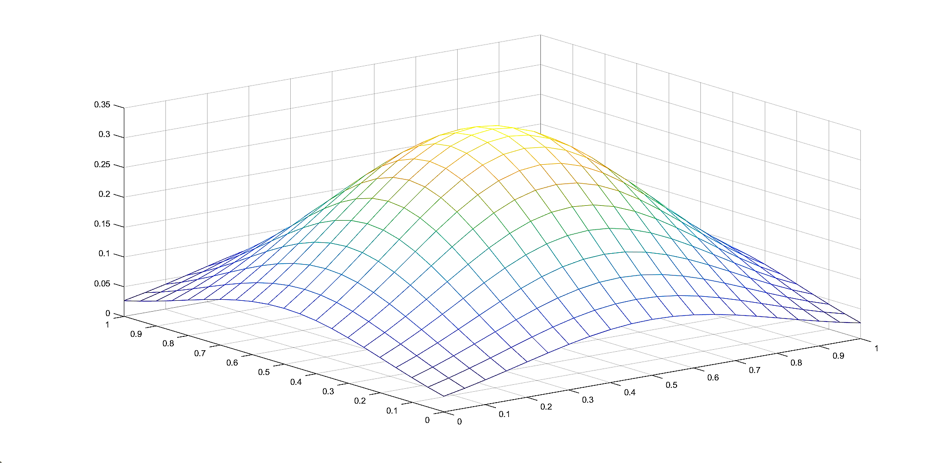
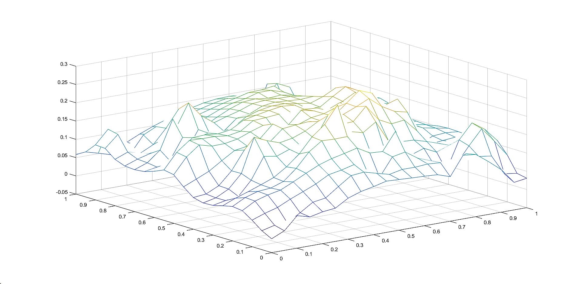
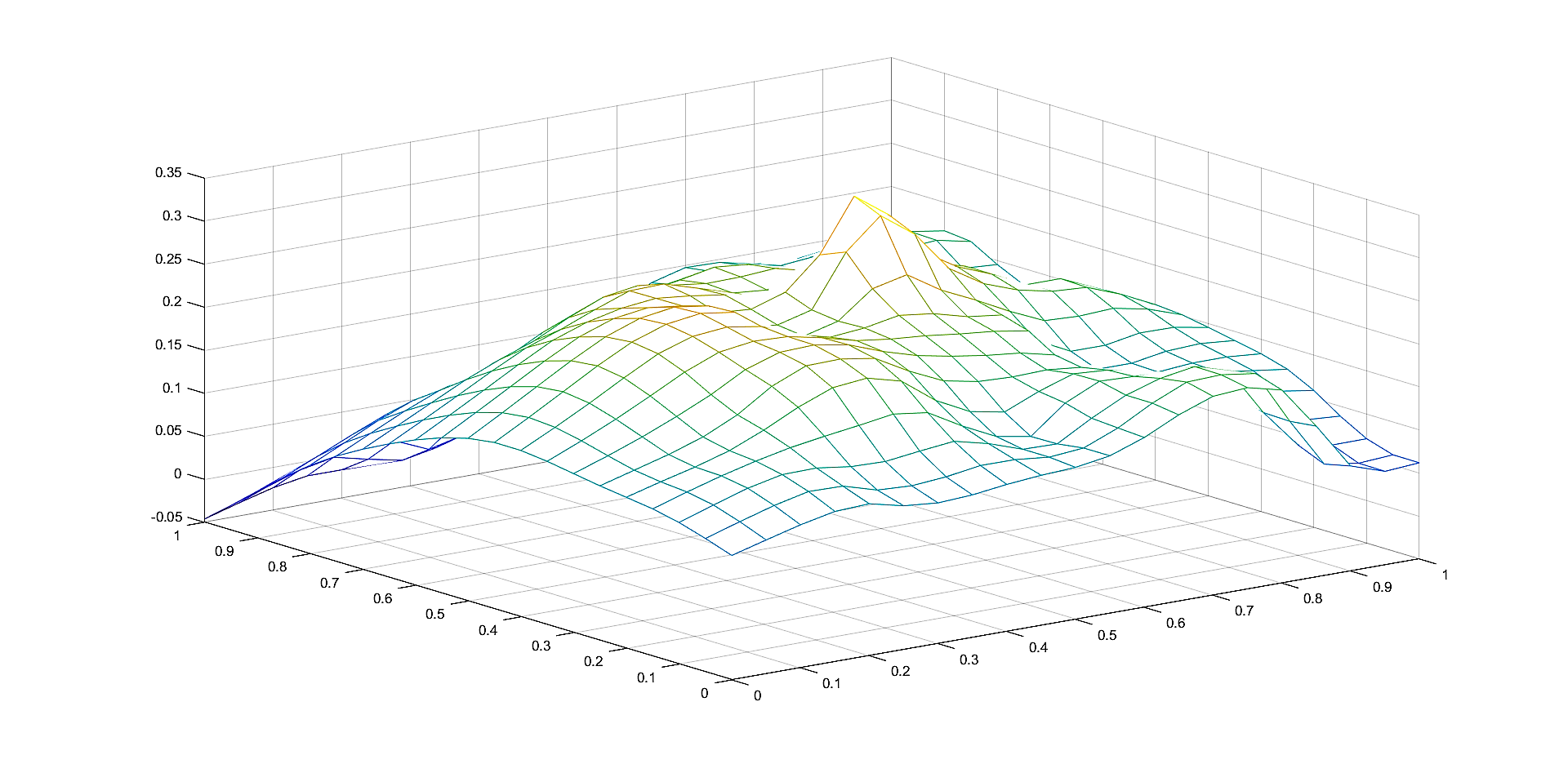
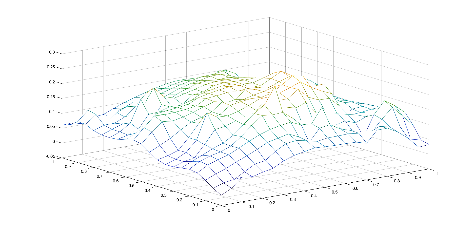
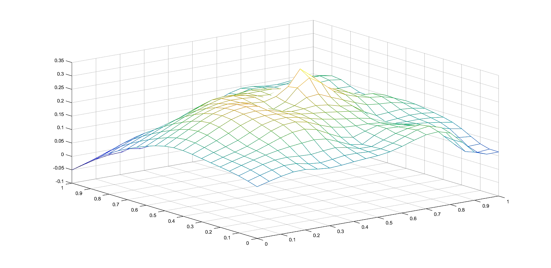
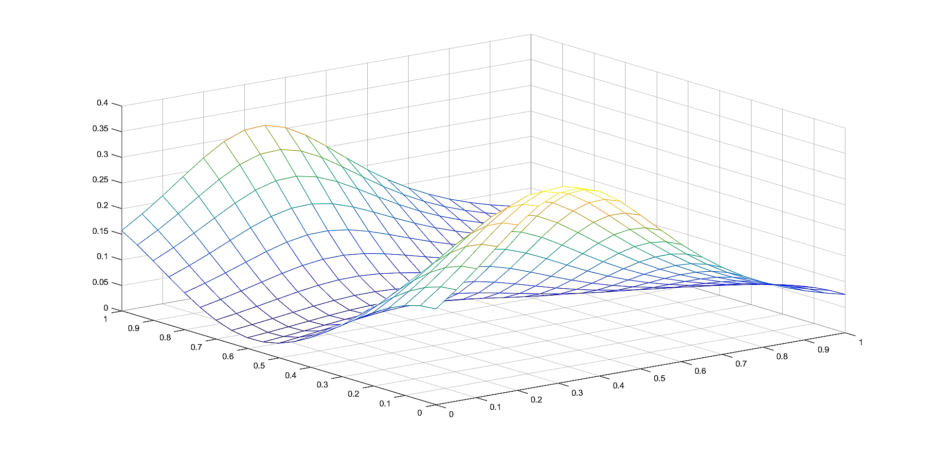
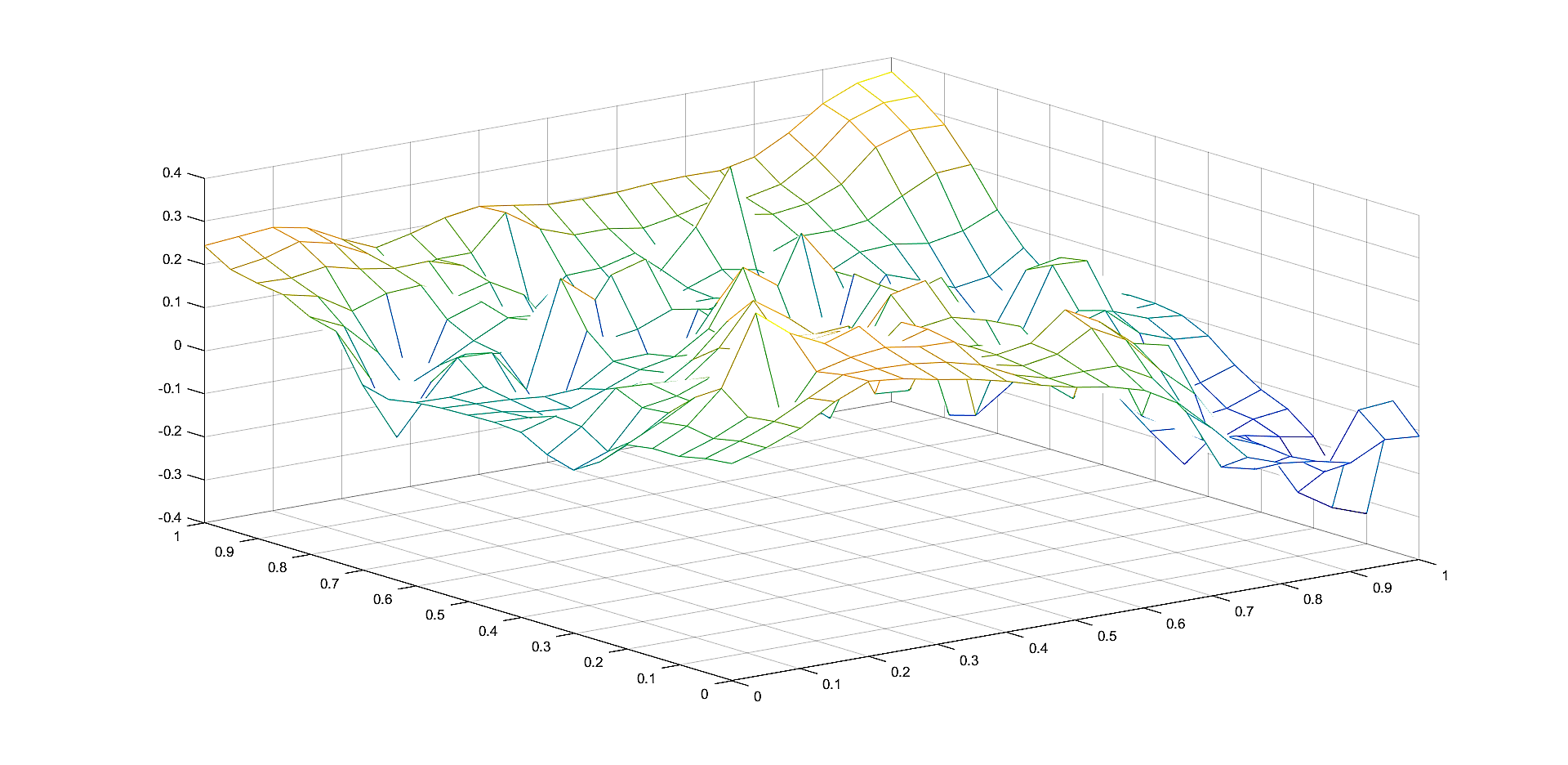
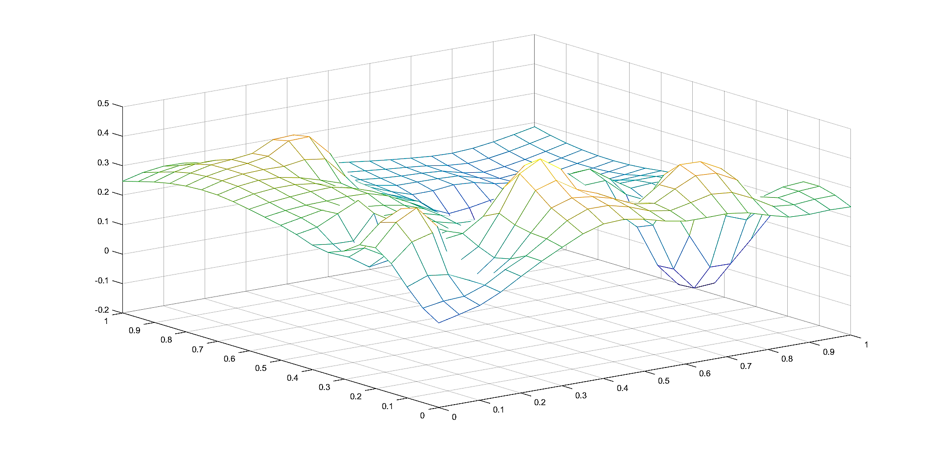
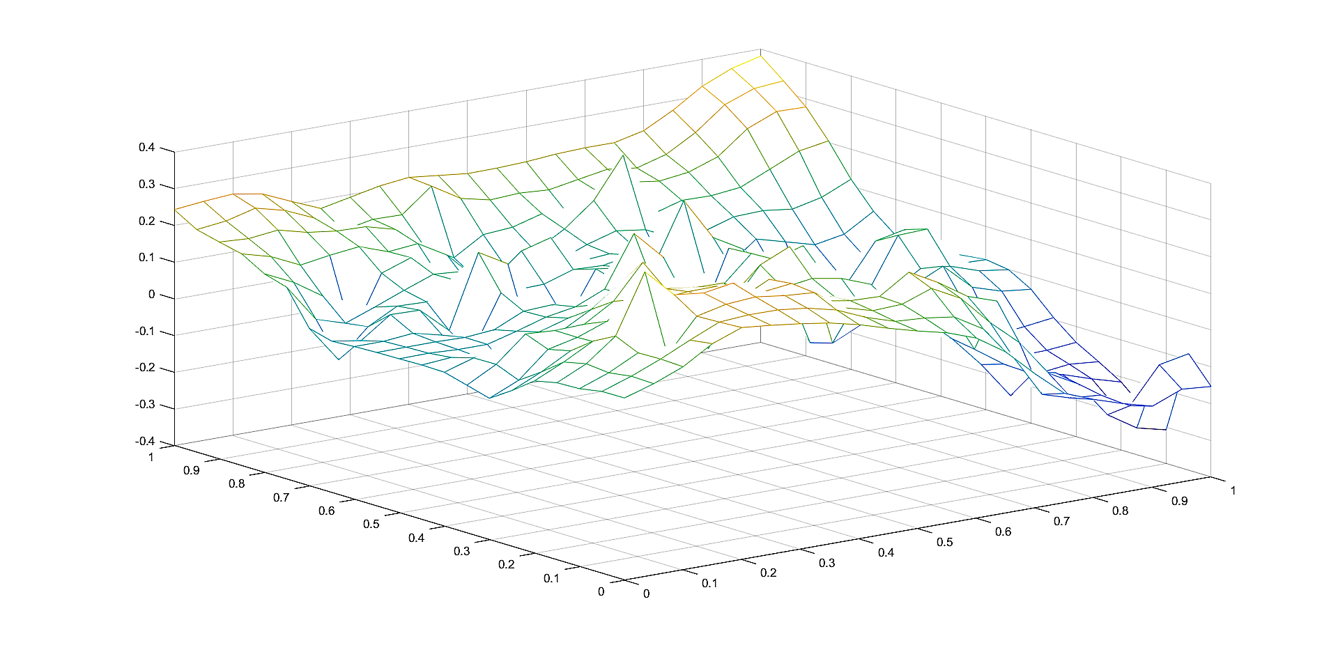
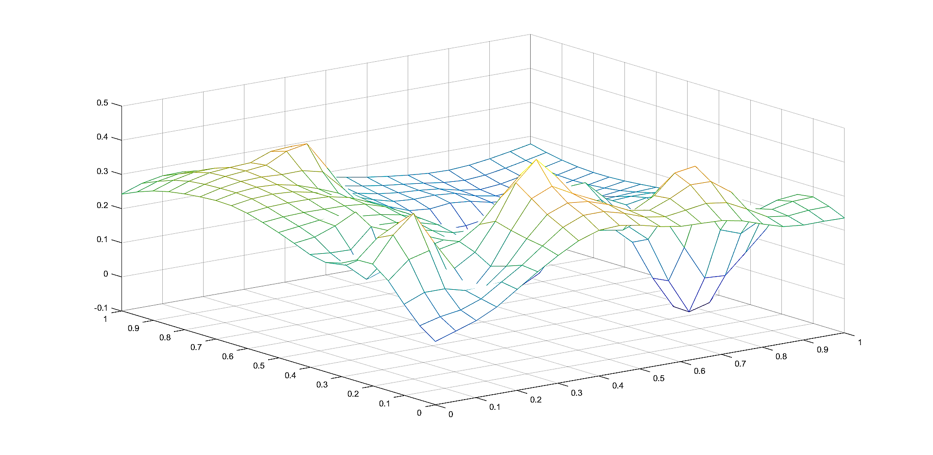
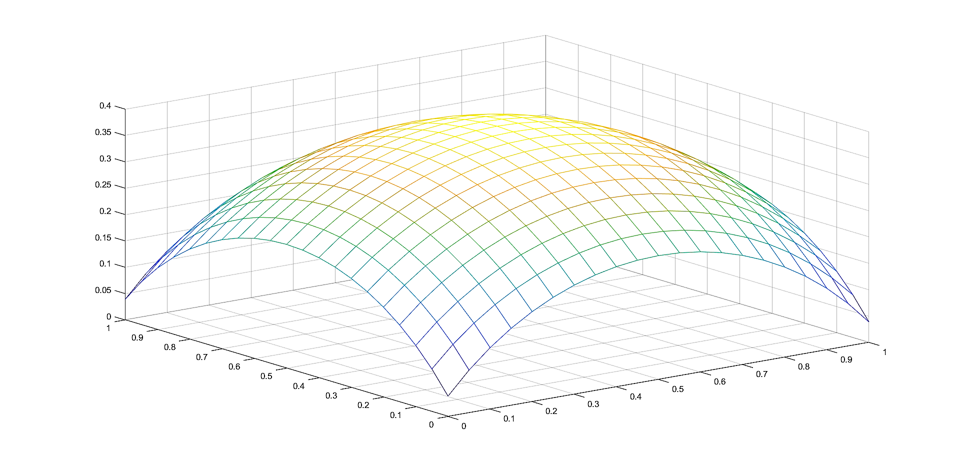
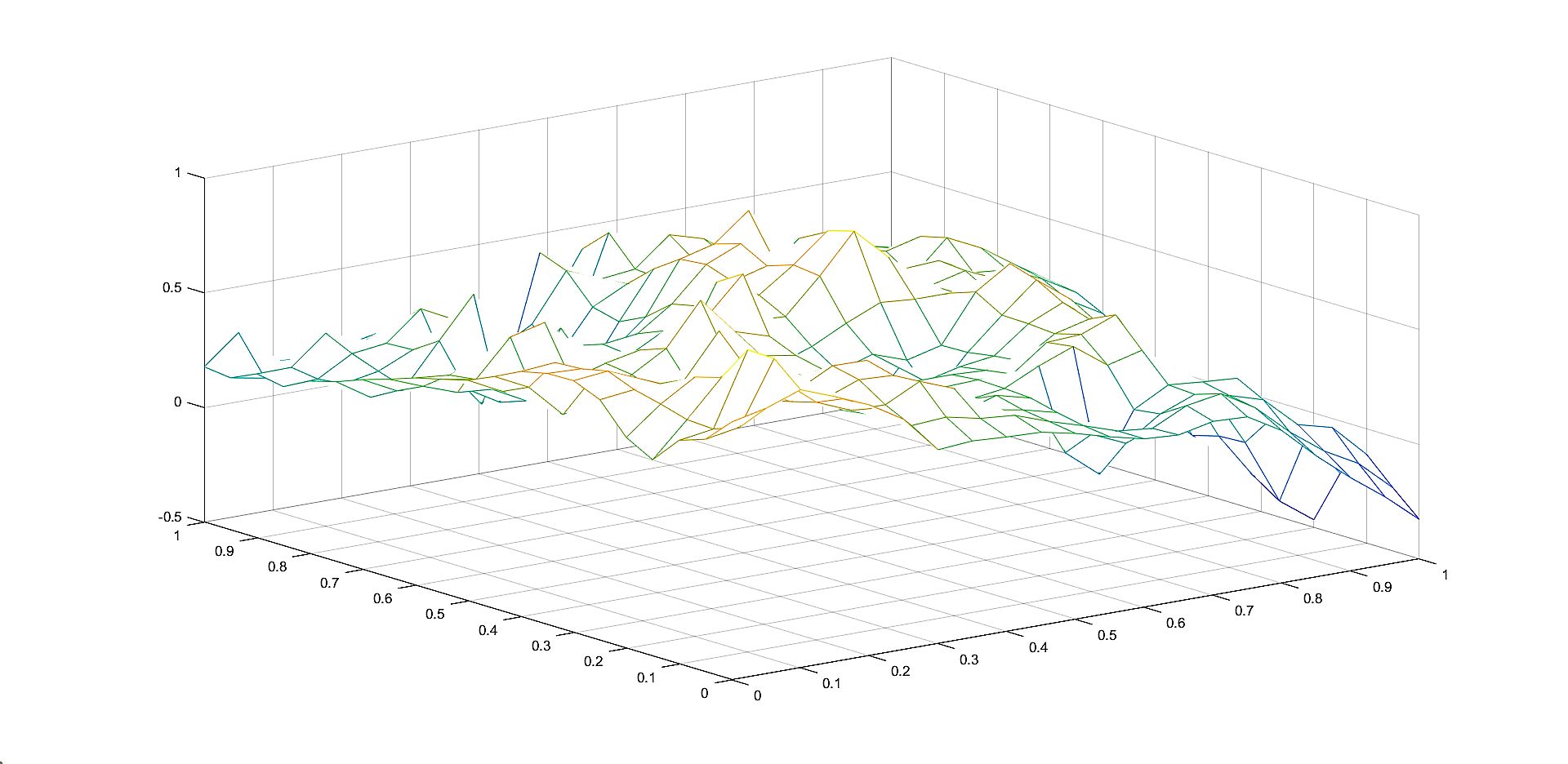
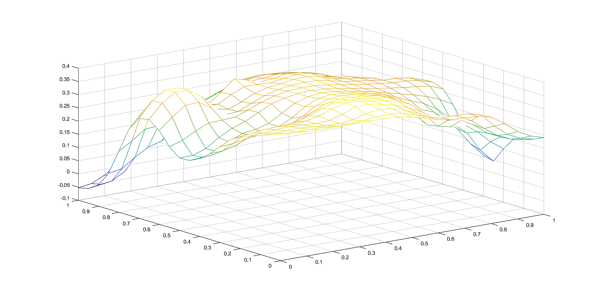
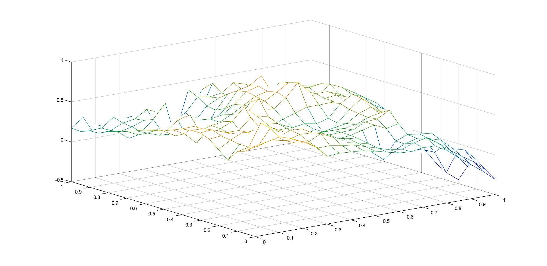
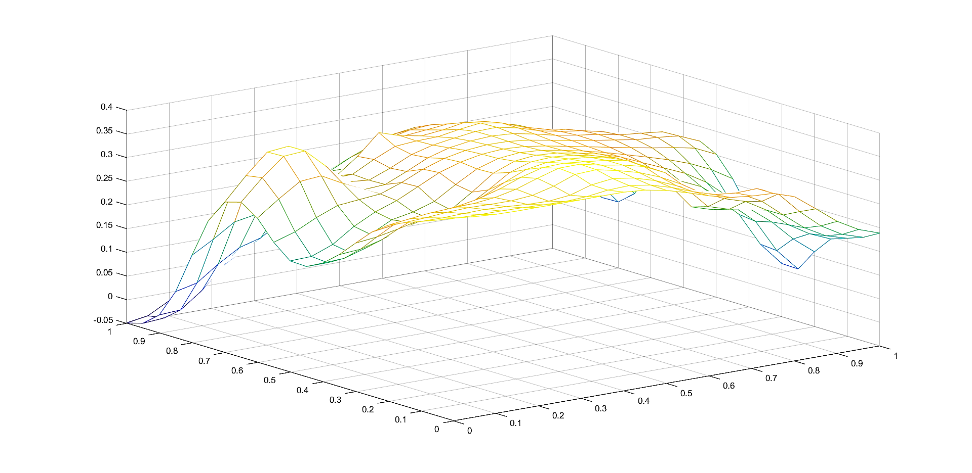
In Figures 2, 4, 6 we plot the graphs of $f_{1},\;f_{2},\;f_{3}$ and of the corresponding Shepard operators $S_{1}f_{i},\;S_{2}f_{i}$ , $S_{3}f_{i}$ and $S_{4}f_{i}$ , $i=1,2,3$ , respectively.

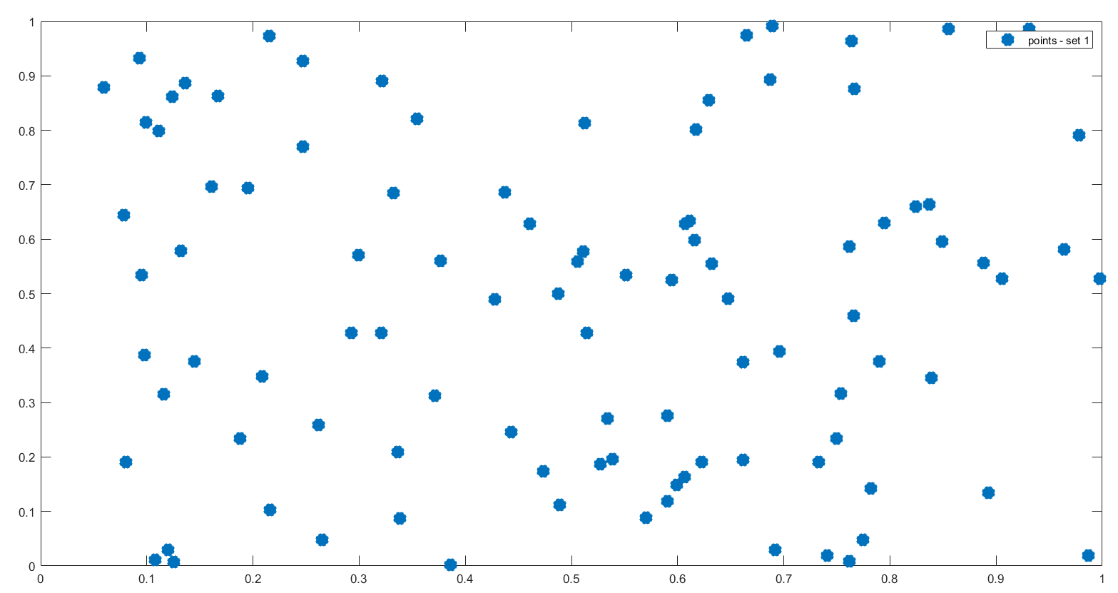
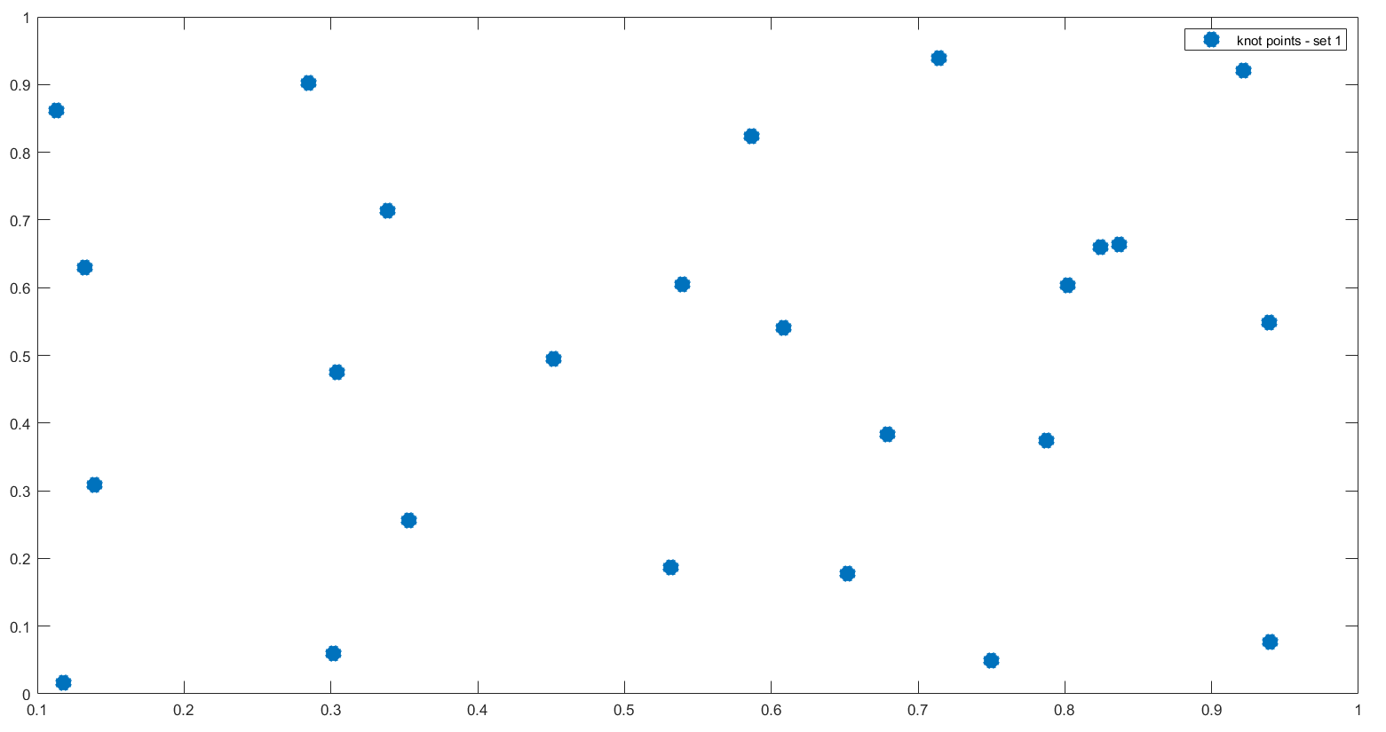
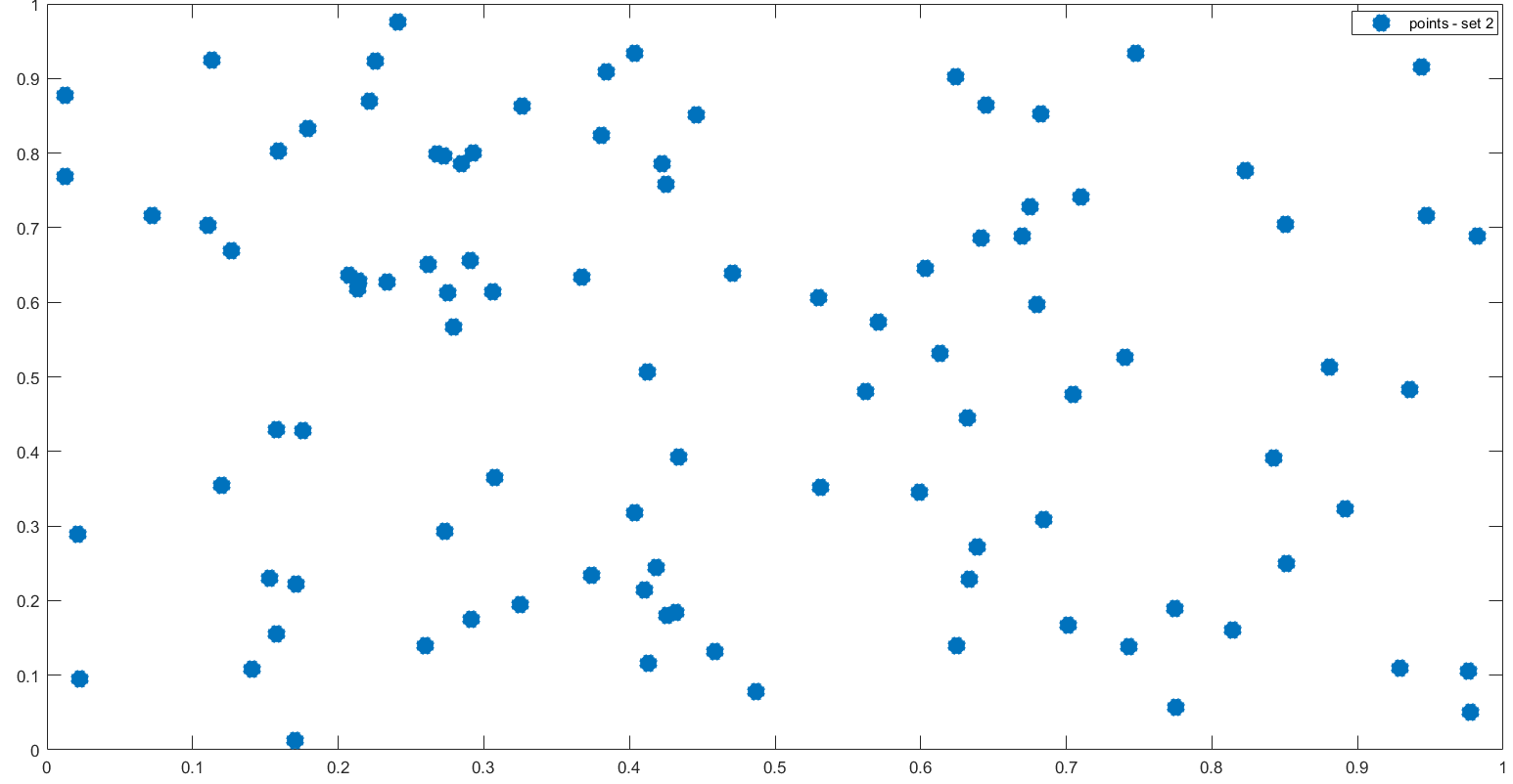
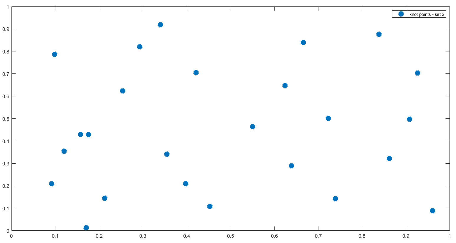
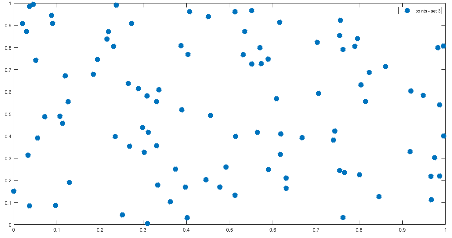
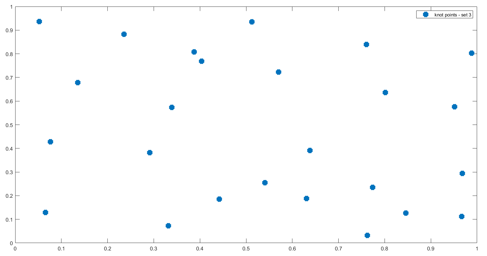
In Figures 1, 3, 5 we plot the sets of the given points and the corresponding sets of the representative knot points.

Table 1. Maximum approximation errors.

	$f_{1}$	$f_{2}$	$f_{3}$
$S_{\mu}f$	0.0864	0.1095	0.1936
$S f$	0.0724	0.0970	0.1770
$S_{1}f$	0.1644	0.4001	0.6595
$S_{2}f$	0.1246	0.2858	0.3410
$S_{3}f$	0.1578	0.3783	0.6217
$S_{4}f$	0.1212	0.2834	0.3399

Refer to caption — First set of given points.

References

[1] Cătinaş, T., The combined Shepard-Abel-Goncharov univariate operator, Rev. Anal. Numér. Théor. Approx., 32(2003), pp. 11–20.
[2] Cătinaş, T., The combined Shepard-Lidstone bivariate operator, In: de Bruin, M.G. et al. (eds.): Trends and Applications in Constructive Approximation. International Series of Numerical Mathematics, Springer Group-Birkhäuser Verlag, 151(2005), pp. 77–89.
[3] Cătinaş, T., Bivariate interpolation by combined Shepard operators, Proceedings of $17^{th}$ IMACS World Congress, Scientific Computation, Applied Mathematics and Simulation, ISBN 2-915913-02-1, 2005, 7 pp.
[4] Cătinaş, T., The bivariate Shepard operator of Bernoulli type, Calcolo, 44 (2007), no. 4, pp. 189-202.
[5] Coman, Gh., The remainder of certain Shepard type interpolation formulas, Studia UBB Math, 32 (1987), no. 4, pp. 24-32.
[6] Coman, Gh., Hermite-type Shepard operators, Rev. Anal. Numér. Théor. Approx., 26(1997), 33–38.
[7] Coman, Gh., Shepard operators of Birkhoff type, Calcolo, 35(1998), pp. 197–203.
[8] Farwig, R., Rate of convergence of Shepard’s global interpolation formula, Math. Comp., 46(1986), pp. 577–590.
[9] Franke, R., Scattered data interpolation: tests of some methods, Math. Comp., 38(1982), pp. 181–200.
[10] Franke, R., Nielson, G., Smooth interpolation of large sets of scattered data. Int. J. Numer. Meths. Engrg., 15(1980), pp. 1691–1704.
[11] Lazzaro, D., Montefusco, L.B.: Radial basis functions for multivariate interpolation of large scattered data sets, J. Comput. Appl. Math., 140(2002), pp. 521–536.
[12] McMahon, J. R., Knot selection for least squares approximation using thin plate splines, M.S. Thesis, Naval Postgraduate School, 1986.
[13] McMahon, J. R., Franke, R., Knot selection for least squares thin plate splines, Technical Report, Naval Postgraduate School, Monterey, 1987.
[14] Renka, R.J., Cline, A.K., A triangle-based $C^{1}$ interpolation method. Rocky Mountain J. Math., 14(1984), pp. 223–237.
[15] Renka, R.J., Multivariate interpolation of large sets of scattered data ACM Trans. Math. Software, 14(1988), pp. 139–148.
[16] Shepard, D., A two dimensional interpolation function for irregularly spaced data, Proc. 23rd Nat. Conf. ACM, 1968, pp. 517–523.
[17] Trîmbiţaş, G., Combined Shepard-least squares operators - computing them using spatial data structures, Studia UBB Math, 47(2002), pp. 119–128.
[18] Zuppa, C., Error estimates for moving least square approximations, Bull. Braz. Math. Soc., New Series 34(2), 2003, pp. 231-249.

[1] Catinas, T., The combined Shepard-Abel-Goncharov univariate operator, Rev. Anal. Numer. Theor. Approx., 32(2003), 11-20.
[2] Catinas, T., The combined Shepard-Lidstone bivariate operator, In: de Bruin, M.G. et al. (eds.): Trends and Applications in Constructive Approximation. International Series of Numerical Mathematics, Springer Group-Birkhauser Verlag, 151(2005), 77-89.
[3] Catinas, T., Bivariate interpolation by combined Shepard operators, Proceedings of 17th IMACS World Congress, Scientific Computation, Applied Mathematics and Simulation, ISBN 2-915913-02-1, 2005, 7 pp.
[4] Catinas, T., The bivariate Shepard operator of Bernoulli type, Calcolo, 44 (2007), no. 4, 189-202.
[5] Coman, Gh., The remainder of certain Shepard type interpolation formulas, Stud. Univ. Babes-Bolyai Math., 32(1987), no. 4, 24-32.
[6] Coman, Gh., Hermite-type Shepard operators, Rev. Anal. Num´er. Th´eor. Approx.,
26(1997), 33-38.
[7] Coman, Gh., Shepard operators of Birkhoff type, Calcolo, 35(1998), 197-203.
[8] Farwig, R., Rate of convergence of Shepard’s global interpolation formula, Math. Comp., 46(1986), 577-590.
[9] Franke, R., Scattered data interpolation: tests of some methods, Math. Comp., 38(1982), 181-200.
[10] Franke, R., Nielson, G., Smooth interpolation of large sets of scattered data, Int. J. Numer. Meths. Engrg., 15(1980), 1691-1704.
[11] Lazzaro, D., Montefusco, L.B., Radial basis functions for multivariate interpolation of large scattered data sets, J. Comput. Appl. Math., 140(2002), 521-536.
[12] McMahon, J.R., Knot selection for least squares approximation using thin plate splines, M.S. Thesis, Naval Postgraduate School, 1986.
[13] McMahon, J.R., Franke, R., Knot selection for least squares thin plate splines, Technical Report, Naval Postgraduate School, Monterey, 1987.
[14] Renka, R.J., Multivariate interpolation of large sets of scattered data, ACM Trans. Math. Software, 14(1988), 139-148.
[15] Renka, R.J., Cline, A.K., A triangle-based C1 interpolation method, Rocky Mountain J. Math., 14(1984), 223-237.
[16] Shepard, D., A two dimensional interpolation function for irregularly spaced data, Proc. 23rd Nat. Conf. ACM, 1968, 517-523.
[17] Trımbitas, G., Combined Shepard-least squares operators – computing them using spatial data structures, Stud. Univ. Babes-Bolyai Math., 47(2002), 119-128.
[18] Zuppa, C., Error estimates for moving least square approximations, Bull. Braz. Math. Soc., New Series, 34(2003), no. 2, 231-249.

2021

On a Volterra Integral Equation with Delay, via w-Distances

October 20, 2021

Approximation of some classes of functions by Landau type operators

May 18, 2021

Kantorovich type operators associated with Jain-Markov operators

July 6, 2021

Shepard operator of least squares thin-plate spline type

Abstract

Authors

Keywords

Paper coordinates

PDF

About this paper

Journal

Publisher Name

DOI

Print ISSN

Online ISSN

MR

ZBL

Google Scholar

Paper (preprint) in HTML form

Shepard operator of least squares thin-plate spline type

Abstract.

Key words and phrases:

1991 Mathematics Subject Classification:

1. Preliminaries

2. The Shepard operators of least squares thin-plate spline type

Method 1.

Algorithm 2.1.

Method 2.

Method 3.

Method 4.

3. Numerical examples

Remark 3.1.

References

References

Related Posts