Abstract
The aim of this paper is to present two algorithms for numerical solving of a fixed final state control problem in connection with the leukemia treatment strategy. In the absence of the controllability condition, our model leads to a nonlinear integral system of Volterra type to whom explicit iterative techniques apply and converge. Once using the controllability condition, the control variable is expressed in terms of the state variables and the integral system changes to a mixed Volterra-Fredholm type one making direct iterative techniques inoperative. However, two paths can be followed. One consists in an iterative procedure where at each step the control variable is calculated using the approximate values of the state variables from the previous step. The other looks for the numerical value of the control variable by using the bisection method. Numerical simulations, error analysis and biological interpretation are given.
Authors
Lorand Gabriel Parajdi
Department of Mathematics, West Virginia University, Morgantown, WV 26506, USA & Department of Mathematics, Babeş-Bolyai University, Cluj-Napoca, Romania
Flavius Pătrulescu
Department of Mathematics, Technical University of Cluj-Napoca, Cluj-Napoca, Romania;
Radu Precup
Faculty of Mathematics and Computer Science and Institute of Advanced Studies in Science and Technology, Babeş-Bolyai University, Cluj-Napoca 400084, Romania
Tiberiu Popoviciu Institute of Numerical Analysis, Romanian Academy, Cluj-Napoca 400110, Romania
Ioan Ştefan Haplea
Department of Internal Medicine, Iuliu Haţieganu University of Medicine and Pharmacy, Cluj-Napoca, Romania
Keywords
Control problem; myeloid leukemia; Volterra-Fredholm integral equation; numerical method.
Paper coordinates
L.G. Parajdi, F. Pătrulescu, R. Precup, I. Şt. Haplea, Two numerical methods for solving a nonlinear system of integral equations of mixed Voltera-Fredholm type arising from a control problem related to leukemia, Journal of Applied Analysis & Computation, 13 (2023) no. 4, pp. 1797-1812, http://doi.org/10.11948/20220197
first page only: http://www.jaac-online.com/article/doi/10.11948/20220197
About this paper
Journal
Journal of Applied Analysis & Computation
Publisher Name
Springer
Print ISSN
Online ISSN
google scholar link
Paper (preprint) in HTML form
Two numerical methods for solving a nonlinear system of integral equations of mixed Volterra-Fredholm type arising from a control problem related to leukemia
Abstract.
The aim of this paper is to present two algorithms for numerical solving of a fixed final state control problem in connection with the leukemia treatment strategy. In the absence of the controllability condition, our model leads to a nonlinear integral system of Volterra type to whom explicit iterative techniques apply and converge. Once using the controllability condition, the control variable is expressed in terms of the state variables and the integral system changes to a mixed Volterra-Fredholm type one making direct iterative techniques inoperative. However, two paths can be followed. One consists in an iterative procedure where at each step the control variable is calculated using the approximate values of the state variables from the previous step. The other looks for the numerical value of the control variable by using the bisection method. Numerical simulations, error analysis and biological interpretation are given.
Key words and phrases:
Control problem, dynamic system, myeloid leukemia, Volterra-Fredholm integral equation, numerical method1991 Mathematics Subject Classification:
45G15, 34H05, 65R20, 92C50, 93B051. Introduction
Human activity in various fields often involves some control over the processes in order to achieve the desired result. Thus, in particular, control intervenes in medicine and is exercised in order to bring the patient to the desired parameters.
The control becomes a mathematical one as soon as a mathematical model is generated for the investigated process by taking into account specific laws such as conservation laws. From a mathematical point of view, the control involves a certain modification of some parameters of the model such that the solution of the problem satisfies a certain requirement.
For such a problem, it is important to demonstrate qualitatively the controllability of the system, i.e., the possibility of achieving the desired goal, but just as important for the implementation of theoretical predictions are the numerical methods designed to provide quantitative results. Therefore, numerical approximation and calculation algorithms are especially important for control problems.
The purpose of this paper is precisely to develop computer-based numerical algorithms for the numerical solution of a control problem related to the treatment of chronic myeloid leukemia. Even if they are presented for a very specific problem, these algorithms can be easily adapted for the numerical treatment of many other classes of control problems.
1.1. Biological Background
Chronic myeloid leukemia (CML) is a slowly progressing malignancy of the blood marrow, derived from the granulocyte cell line. Left untreated, it causes moderate symptoms on its own, but can nonetheless progress over years to aggressive, life-threatening forms (accelerated or blast phase) (see E. Jabbour and H. Kantarjian [1]). The molecular culprit (and hallmark) of CML is the oncoprotein BCR-ABL1, generated by an abnormal fusion of two genes, which normally belong to distinct chromosomes. BCR-ABL1 has intrinsic tyrosine kinase activity and switches the molecular machinery of cell signal transduction to an ”always on” state. This increases cell division and proliferation, largely irrespective of stimulation by growth factors and confers a malignant phenotype (see S. Faderl et al. [2]).
Frontline therapy for CML relies on tyrosine kinase inhibitors (TKI). These are targeted anticancer drugs, designed to block the BCR-ABL1 protein, specifically, potent and selective enough to drive the leukemic cell population closer to extinction while sparing the normal granulocyte line. From the first molecule (Imatinib, see S.G. O’Brien et al. [3]), TKIs have diversified to date to second and third generation agents, with increased potency. All TKIs are very effective in treating CML, with rates of major response at 10 years approaching 95% (see A. Hochhaus et al. [4]).
The state of the disease and the response to treatment are monitored primarily by the number of mARN copies of the BCR-ABL1 gene, as measured by qRT-PCR from the patient’s blood, normalized to a control (see T. Hughes et al. [5]). Presently, the life expectancy of patients with CML approaches the average of the general population, especially in developed countries (see M.W. Deininger et al. [6]). In addition to survival, the focus of research in CML is quality of life, the effect of comorbidities, toxicity profile of TKI, and the discontinuation of drugs once major treatment milestones have been met (see A. Hochhaus et al. [7]). These concerns are especially prominent since the median age of CML onset is close to 70 years of age. The side effects of TKIs can be mitigated by dose reduction (for Imatinib, from 400 mg per day to 300 mg per day) or a brief drug holiday.
All these suggest the necessity for an optimized and theoretically grounded dosing schedule in CML that reaches the treatment targets in an efficient yet parsimonious way. We have explored the problem of TKI dosing in CML by a quantitative dynamical model.
1.2. Mathematical Model and Approach
Over the years, many mathematicians and biologists have proposed and studied different types of models and problems inspired by life phenomena, such as Y. Cherruault [8], C.J.S. Alves et al. [9], Y. Wang et al. [10] and G. Cedersund et al. [11]. From the numerous works in which there are studied optimization problems and control problems applied to chronic myeloid leukemia (also known as chronic myelogenous leukemia), we mention those of S. Nanda et al. [12], B. Ainseba and C. Benosman [13], Q. He et al. [14], S.B. Mendrazitsky and B. Shklyar [15] and S.B. Mendrazitsky et al. [16].
In a paper of M.C. Mackey and L. Glass [17], it is introduced a mathematical model of blood production using differential equations involving sigmoid or Hill functions, given the fact that hematopoiesis is a self-limiting process. Based on this model of blood production from Mackey-Glass [17], in L.G. Parajdi et al. [18] it is considered the following mathematical model
| (1.1) |
where are the normal and leukemic cell populations at time , respectively. Here, the parameters are the growth rates; are the cell death rates (or cell turnover rates); and are the sensitivity parameters that govern the self-limiting process. For both cell populations, we assume that the growth rate is greater than the death rate, i.e., and . The eventual advantage of leukemic cells of being less sensitive to the microenvironment than normal cells is expressed by
The case , was studied by Dingli and Michor [19] (see also the paper of A. Cucuianu and R. Precup [20]), in order to describe the time competition between normal and leukemic hematopoietic stem cells. In this case, there exist only two non-zero steady states and of the system, where and represent the homeostatic amounts of normal and leukemic (or abnormal) cells and are given by
The case , was introduced and studied in the paper of L.G. Parajdi et al. [18] and the book of L.G. Parajdi [21]. In this case, besides the two non-zero steady states , there could also exist a third steady state , where
We can observe that under the assumption , both and are positive if and only if The case when corresponds to the normal hematologic state, the case corresponds to the chronic phase of the disease, and the case stands for the acute/blast phase. In the first case (normal state), system (1.1) has the unique stable equilibrium , in the second case (the chronic phase) the stable equilibrium is of the form , where both and are positive, and in the third case (the acute/blast phase) the stable equilibrium is .
In this paper, we give two numerical methods for solving a nonlinear system of integral equations of mixed Volterra–Fredholm type, arising from a control problem related to myeloid leukemia. This system of integral equations, presented in Section 2, is related to the control problem where the control is a constant (connected to a constant drug dose) intended to decrease the growth rate of malignant cells. The model could be related to targeted therapies. This control problem was introduced and studied in the paper of I.Ş. Haplea et al. [22] and its analysis, reproduced in Section 2, is based on a new method for the controllability of abstract fixed point equations. The stability of the control problem is also reminded. In Section 3, we introduce and describe two algorithms that are used to approximate numerically the solution of the integral system. In this context, by Theorem 3.2, it is proved the continuous dependence of the solution on the control parameter, and by Theorem 3.3, the convergence of our first algorithm. Numerical simulations and error analysis are then performed to illustrate the theoretical results and prove their applicability. Finally, in Section 4, we discuss the biological significance of our theoretical and numerical results.
2. A Control Problem for the Normal-Leukemic System
The control problem that is considered in this paper is inspired from hematology, more exactly from the treatment of the chronic phase of chronic myeloid leukemia (CML). It was introduced and studied in I.Ş. Haplea et al. [22] and directly folds on the general control problem for differential systems as stated in V. Barbu [23] (page 34). In this section, we recall the general problem of control theory, the general controllability principle, and a result about the stability of the control problem. All these notions and results are stated in terms of fixed point theory.
2.1. A General Controllability Principle
Consider a general control problem that consists in finding a solution to the following system
| (2.1) |
where is the state variable, denotes the control variable, is the domain of the states, represents the domain of controls and finally, is the controllability domain, usually given by means of some condition imposed to or to both and Therefore we take into consideration a general formulation of the control problem, only in terms of sets, since and are not necessarily structured sets and is any mapping from to .
We say that the equation is controllable in with respect to , if problem (2.1) has a solution.
Let be the set of all possible solutions of the fixed point equation and be the set of all that are the first components of some solutions of the fixed point equation, that is
Obviously, the set of all solutions of the control problem (2.1) is given by
Consider the set-valued map defined as
We have the following general principle for solving the control problem (2.1).
Proposition 2.1.
If for some extension of from to there exists a fixed point of the set-valued map
i.e.,
for some then the couple is a solution of the control problem (2.1).
Remark 2.1.
In particular, and can be single-valued maps.
The above general principle of controllability can be applied to control problems related to the normal-leukemic system.
2.2. A Control Problem for the Normal-Leukemic System
Consider as a condition of controllability, the decrease to a certain acceptable level of the malignant cell population and as a control variable, the factor of decreasing the proliferation rate of cancer cells. Therefore, we consider the following initial value problem
| (2.2) |
where represents the control parameter.
Let us change the variables as follows:
and denote
Dividing the first equation by and the second equation by in the system (2.2), and then integrating, we obtain the integral system equivalent to the initial value problem (2.2), namely
| (2.3) |
This is our fixed point equation where and
The objective condition associated to the integral system (2.3) is
| (2.4) |
where is the expected level of leukemic cells after a period of time .
The biological interpretation is the following: the system
(2.2) extends the basic system (1.1) by adding the effect
of the treatment. We have assumed that TKIs, being a targeted drug,
acts exclusively on the malignant cell (absolute specificity), and
solely by decreasing the proliferation rate of malignant cells (from
to , where is a positive subunit quantity, i.e., )
(see F. Michor et al. [24]). A smaller value for
translates to a more efficient treatment (a higher dose or a more
potent drug). The parameter stands for the effect of TKI
on the growth rate of malignant cells, rather than the actual drug
dosage; is completely determined by the drug dosage but
relates to it in a nontrivial way. As a simplification, we have
assumed a dosing scheme that maintains the drug effect
constant, for the whole duration of the treatment; as such, all
pharmacokinetic details could be safely excluded from the analysis. The
goal of the optimization procedure is to reach the desired (very
low) number of malignant cells, after a given treatment time ,
. This is qualitatively in line with current clinical
guidelines, which prescribe that BCR-ABL1 transcript levels should
be reduced strongly after 12 months of treatment (major molecular
response, MMR) and, in the long run, be brought next to or below
detection levels (deep molecular remission, DMR)
(see the ESMO Clinical Practice Guidelines: A. Hochhaus et al. [25]).
Compared with the abstract general controllability principle from the previous subsection, here we have
and the integral system (2.3) stands for the fixed point equation , with .
We recall the following controllability result obtained using the general principle given by Proposition 2.1 from I.Ş. Haplea et al. [22]. This result shows the solvability of the control problem (2.3)-(2.4).
Proof.
Let , that is which solves (2.3) for some . From the second equation of (2.3) and using the controllability condition (2.4), we obtain
| (2.5) |
We consider a function given by
Next, we can extend this function from to by using the same expression, namely
for . We note that and are single-valued maps.
Thus, our fixed point equation with , becomes
| (2.6) |
which is a system of mixed Volterra–Fredholm type integral equations, where
The existence of a fixed point of can be guaranteed by using Schauder’s fixed point theorem (see R. Precup [26], page 33). Indeed, the operator is completely continuous, as follows immediately from the Arzelà–Ascoli theorem (see R. Precup [26], pages 2, 3 and 15). On the other hand, we have
Consequently, there are numbers with
for all Hence, where
Thus, Schauder’s fixed point theorem applies and guarantees the existence in of a fixed point of Finally, the control is calculated using formula (2.5) with and thus determined.
∎
Remark 2.2.
Since (2.3) is a Volterra system with Lipschitz continuous nonlinearities, for any given , it has a unique solution In particular, for the value corresponding to a solution of the control problem, the trajectory is unique. We may interpret this fact in the following way: for a prescribed drug dose, the patient’s evolution is uniquely determined.
2.3. Stability of the Control Problem
Let us also mention the following stability result of the control problem given in I.Ş. Haplea et al. [22].
Theorem 2.3.
In its proof, there are used Lipschitz estimates and Gronwall’s inequality in order to obtain the estimate
| (2.7) |
which in view of the expression of , immediately implies
Remark 2.3.
Estimate (2.7) shows us that for a treatment close enough to the prescribed treatment the patient’s evolution remains in the vicinity of the prescribed evolution
Note that, due to this stability result, the actual administration of only an approximate dose leads, however, to a result close to the expected one. The level of freedom to choose an approximate dose is exactly established in terms of model parameters.
3. Numerical Algorithms
In this section, we introduce our numerical algorithms for solving problem (2.3)-(2.4) which can be put under the form of the Volterra-Fredholm integral system (2.6). At any step of each one of the two algorithms, we need to solve numerically a Volterra type integral system and this is done with the Picard-Lindelf iteration technique (see E. Hairer et al. [27]) combined with the successive approximation method. The description of the algorithms is followed by some implementation details. Finally, some numerical results in the form of tables and figures are given, and their biological interpretation is the subject of the discussion section, Section 4. All numerical simulations were carried out on the Kotys HPC (High Performance Computing) infrastructure of ”Babeş–Bolyai” University of Cluj-Napoca (see D. Bufnea et al. [28]), using MATLAB software.
3.1. The First Algorithm
In this subsection, we introduce our first algorithm. Therefore, we prove the continuous dependence result, see Theorem 3.2, using the definition of the Bielecki norm and the definition of the spectral radius plus the lemma of convergence of the power sequence of a matrix, all mentioned below.
Definition 3.1.
Let be a Banach space, where , we have the Bielecki norm as follows:
Definition 3.2.
The spectral radius of a square matrix is
For an matrix let .
Lemma 3.1.
Let be a square matrix, with spectral radius If , then . On the other hand, if , then . The statement holds for any choice of matrix norm.
Proof.
We recall that the matrix for a matrix in the Jordan normal form and regular matrix , and we know that . Next, if , then converges to the zero matrix, and thus converges to the zero matrix as well. If , then has a diagonal entry for an eigenvalue such that , and if is the -th column of and the -th row of , then . Therefore, , and thus . ∎
Theorem 3.2.
The solution of system (2.3) depends continuously on parameter .
Proof.
We denote by and the components and of the solution that corresponds to . From the integral system, using the Lipschitz continuity of the nonlinearities and the Volterra property of the equations, we deduce the estimates of the form
and
Here denotes the Bielecki norm on with respect to a sufficiently large . Moreover, represents some constant and the spectral radius of matrix is subunitary, i.e.,
It follows that
or, equivalently,
where are the entries of the matrix . Clearly, from these inequalities, we may conclude the Lipschitz continuity on of the solution.
∎
Next, we assume that the following conditions hold
From a biological point of view, this is a rational assumption meaning that the target value for the leukemic level is chosen below the level that would occur in the absence of any control and is above the level corresponding to a hypothetical zero growth rate of leukemia cells.
Taking into account the above arguments, we define the following
iterative algorithm. It is aimed to bring us as close as
possible to a value of that corresponds to a solution of the control problem.
Step. 1.1. We initialize ,
Step. 1.2. At any iteration we define and solve system (2.3) for . The numerical solution is obtained
where and are given in the proof of Theorem 3.2.
If then put , ,
otherwise, we take , .
Step. 1.3. The algorithm stops if
where . Otherwise, it continues with Step 1.2.
Concerning the above algorithm, we have the following convergence result.
Theorem 3.3.
Proof.
For we have the solution corresponding to . Moreover, we have if or if , where and are the operators defined in the proof of Theorem 3.2. Therefore, we obtain an increasing sequence () and a decreasing sequence () with the following properties
| (3.1) |
and
| (3.2) |
The two sequences being monotone and bounded are convergent. Moreover, from (3.2) they have the same limit . Using the continuity of with respect to and (3.1) we deduce that
| (3.3) |
Finally, we use again the continuity of the operators and with respect to to obtain and . These together with (3.3) show that is a solution of the control problem (2.3)-(2.4).
∎
Further, we provide some computational details concerning the implementation of this algorithm. More exactly, we consider the following -point discretization of the interval
and we define the following subsets
We mention that at Step 1.2 we must solve, for each , a system of nonlinear Volterra integral equations, namely
To this end, we introduce the notation for a general quadrature formula that uses the nodes from , i.e,
where and represent the coefficients. Moreover, we denote by the numerical approximations of at the point , where and . They are the solutions of the nonlinear systems
In the case of the trapezoidal rule for equidistant nodes, the previous systems take the form
| (3.4) |
where
and denotes the constant length between discretization points, i.e., . To solve the nonlinear systems (3.4) we can use a specific numerical method, such as the method of successive approximations.
3.2. The Second Algorithm
In this subsection, we propose a second algorithm which has the following structure.
Step. 2.1. We consider two start functions satisfying
Step 2.2. Using (2.5) we compute
Step 2.3. We solve Volterra system (2.3) for and obtain its solution
Step 2.4. The algorithm stops if the following conditions are satisfied
where . Otherwise, there are performed Steps 2.2 and 2.3 for , .
3.3. Numerical Results
We finish this section with some numerical results which are illustrated in the figures below and whose biological analysis is given in the next section. The numerical results are obtained using a grid with equidistant points. We use the trapezoidal method and we take in the stop condition. Concerning the parameters, the following values are taken (see I.Ş. Haplea et al. [22]):
while for we consider values from the interval .
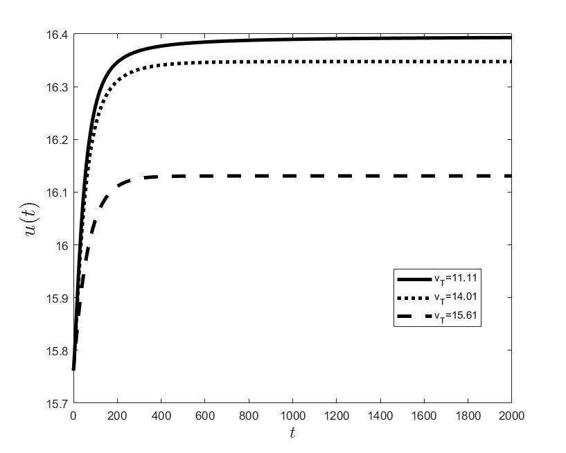
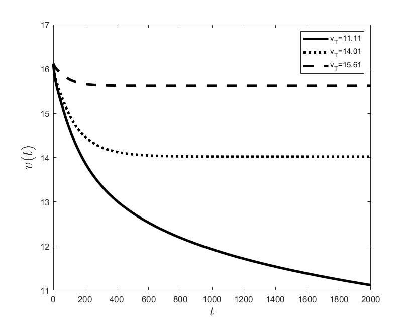
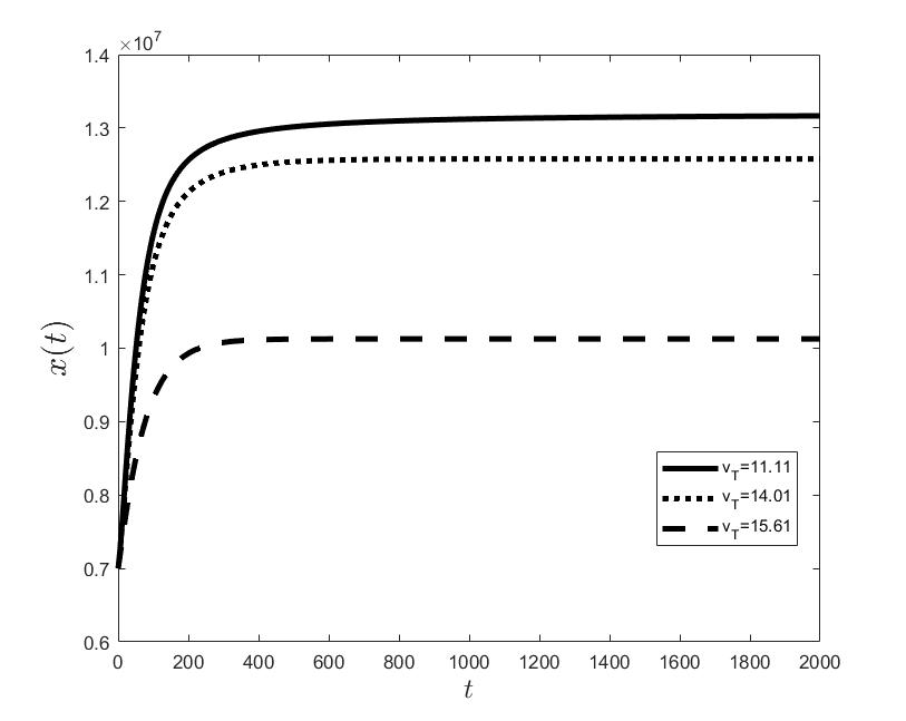
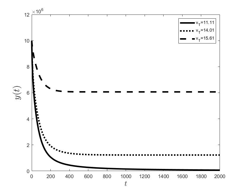
Figures (a) and (b) give the graphs of the functions and for . Notice the asymptotic behavior of these functions and their inverse monotony with respect to Indeed, at any time , the value decreases and the value increases as the target value decreases.
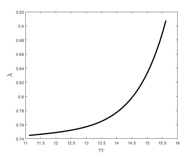
Figure (c) shows the variation of the control parameter with respect to .
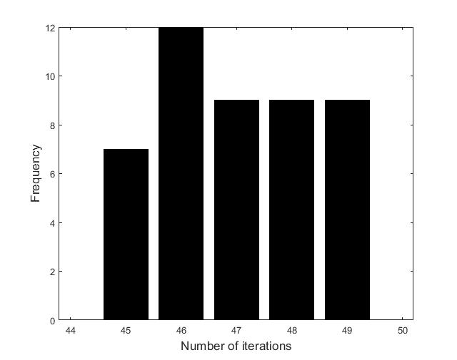
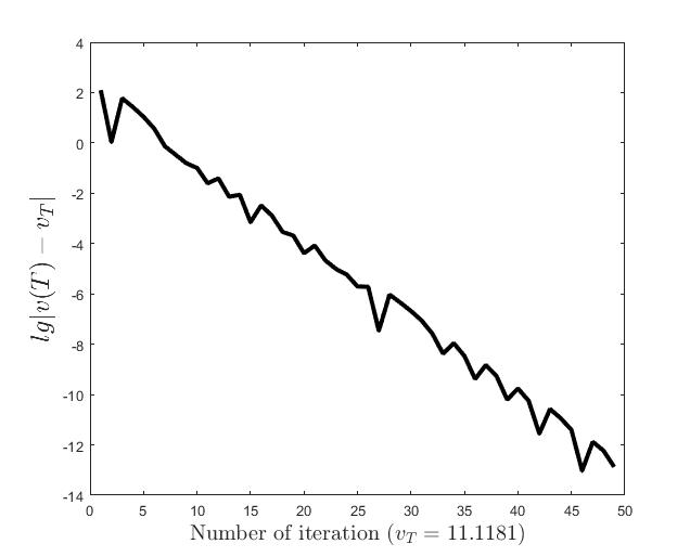
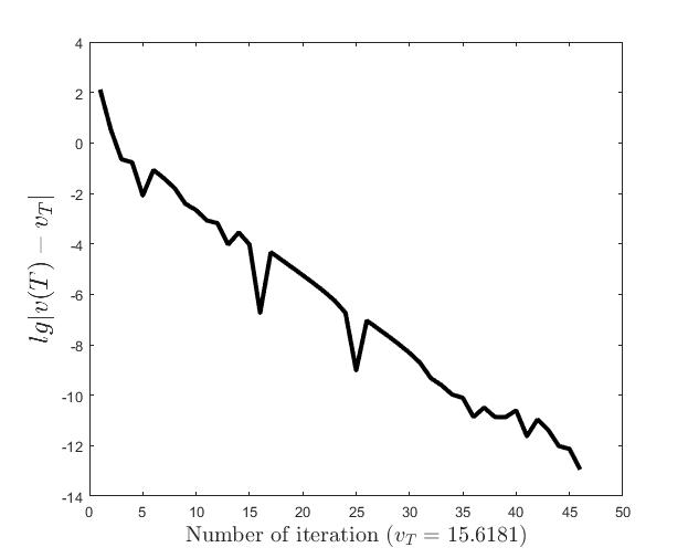
Figures (d)-(f) have the role to give some details about the efficiency of the algorithm Step 1.1-Step 1.3. Thus, the histogram in Figure (d) shows the frequency of the number of iterations in Step 1.2 necessary to solve the nonlinear integral system, in the case when takes equidistant values in the interval , that is when the difference between two consecutive values of is constant and equal with . It is observed that around iterations are necessary to reach the desired error, i.e., .
Figures (e) and (f) show the behavior of the error with respect to the number of iterations, for and .
In Figures (g) and (h), there are represented the graphs of functions and . Some biological considerations about them are given in the next section.
Finally, we mention that similar results are obtained using the second algorithm Step 2.1 -Step 2.4. In this case, the number of iterations strongly depends on the start functions taken in Step 2.1. Also, the approximation of in Step 2.2 increases the complexity of the algorithm. However, in contrast to the first algorithm, the error decreases in a monotone manner.
.
.
.
.
4. Discussion
The results of the numerical simulations (Figures (b) and (h)) agree with the data of CML cases treated with TKIs (see M.C. Müller et al. [29] and F. Michor et al. [24]); malignant cell counts decrease monotonically in time, with a sharp decline for the first to time units (days of treatment), followed by a slower phase that eventually plateaus out. Normal cells expand in compensation (Figures (a) and (g)). As expected, the more stringent the target (a lower ), the longer it takes to approach and converge to it (Figure (h)). To answer the question: what drug effect is required to suppress the malignant population down to a given level, we have explored numerically the relationship between and (Figure (c)). We have found a monotonic relationship, where increases faster than linearly with , and in consequence incrementally larger drug loads are required for every additional unit of reduction in the malignant cell population. This confirms that hematological cure by dose escalations alone can be prohibitively costly in terms of drug toxicity for unresponsive patients, and alternative management (like switching to an alternative TKI) is best considered in such cases.
Normal and leukemic cell populations are internally structured, with subpopulations of stem, progenitor and variably differentiated cells. We have collated all the cell subtypes within a single normal cell phenotype and another single malignant cell phenotype. Also, myeloid leukemias develop functionally in two compartments, the hematopoietic bone marrow and the peripheral blood. While the bone marrow (the production compartment) is severely space constrained, the more compliant circulatory blood can accommodate massive increases in myeloid cell counts. These increases range from severalfold (physiologically) to almost two orders of magnitude (pathologically) (see J. Gong et al. [30]). In our model, we have compacted the generative central (medullary) compartment and the transit peripheral (blood) compartment in a single compartment. This amounts to assuming constant rates of cell transport between compartments. While the numbers of modeled cells, normal and malignant, need not add up to a constant ( can vary in time), there is an implicit pressure in the model toward lower counts through allo- and hetero feedback. This is in qualitative accord with actual biology, as even the bone marrow has some margin for variable cell density (histologically, it can be of ”higher” or ”lower cellularity”).
In current hematology practice, the CML state is assessed by the ratio of BCR-ABL1 transcripts to ABL1 transcripts, rather than by the absolute levels of BCR-ABL1. We have departed from this standard, as we have chosen for the goal of the optimization, the absolute number of leukemic cells . This makes our method more general, as it is readily extendable to solid malignancies where absolute cell counts can be derived from imaging studies.
The goal of CML treatment with TKIs is to achieve long-term molecular remission. Earlier evaluations at shorter terms ( and months of treatment) serve only to predict the long-term response (see B. Hanfstein et al. [31]), but otherwise have no clinical utility on their own. If the treatment fails to lower BCR-ABL1 enough at three months, the patient is classified as a nonresponder and switched to an alternative, likely more efficient TKI. Imatinib (a first-generation molecule) is the agent most often used as a first-line for CML, while the more potent second and third-generation TKIs may be withheld due to the cost and toxicity profile. A direction for future research is to model the treatment with different TKIs in succession, each with its specific value, and to identify the optimal time points of the switch from one drug to the other, in view of some goal of persistent remission.
In the work I.Ş. Haplea et al. [22] we have also optimized the (modeled) treatment of acute leukemia, using as a control objective the whole timecourse of the disease under treatment (i.e., the leukemic cells should decrease along a predefined curve), which reflects the need to monitor tightly an acute disease. For chronic leukemia, it appears reasonable to use solely the long-term endpoint as a goal. Nonetheless, as the existence of the solution has been proved for the chronic form, the endpoint will be reached, in every case, along a single uniquely determined curve. It would be of interest to check the form of the so-established curve against the intermediate targets from clinical guidelines. Our model may predict that the final target can be attained even if early targets are not met. Both coincidence or disparity between the model and reality would lead to some insight.
Acknowledgment:
The authors would like to thank the reviewers for their careful reading of the manuscript and for their valuable comments and suggestions.
L.G. Parajdi benefited from financial support through the project ”The Development of Advanced and Applicative Research Competencies in the Logic of STEAM+ Health”, POCU/993/6 /13/153310, a project co-financed by the European Social Fund through The Romanian Operational Programme Human Capital 2014-2020.
References
- [1] E. Jabbour and H. Kantarjian, Chronic Myeloid Leukemia: 2020 Update on Diagnosis, Therapy and Monitoring. Am. J. Hematol. 95 (6) (2020), 691–709.
- [2] S. Faderl, M. Talpaz, Z. Estrov, S. O’Brien, R. Kurzrock and H.M. Kantarjian, The Biology of Chronic Myeloid Leukemia. N. Engl. J. Med. 341 (3) (1999), 164–172.
- [3] S.G. O’Brien, F. Guilhot, R.A. Larson, I. Gathmann, M. Baccarani, F. Cervantes, J.J. Cornelissen, et al., Imatinib Compared with Interferon and Low-Dose Cytarabine for Newly Diagnosed Chronic-Phase Chronic Myeloid Leukemia. N. Engl. J. Med. 348 (11) (2003), 994–1004.
- [4] A. Hochhaus, R.A. Larson, F. Guilhot, J.P. Radich, S. Branford, T.P. Hughes, M. Baccarani, et al. Long-Term Outcomes of Imatinib Treatment for Chronic Myeloid Leukemia. N. Engl. J. Med. 376 (10) (2017), 917–927.
- [5] T. Hughes, M. Deininger, A. Hochhaus, S. Branford, J. Radich, J. Kaeda, M. Baccarani, et al., Monitoring CML Patients Responding to Treatment with Tyrosine Kinase Inhibitors: Review and Recommendations for Harmonizing Current Methodology for Detecting BCR-ABL Transcripts and Kinase Domain Mutations and for Expressing Results. Blood 108 (1) (2006), 28–37.
- [6] M.W. Deininger, N.P. Shah, J.K. Altman, E. Berman, R. Bhatia, B. Bhatnagar, D.J. DeAngelo, et al., Chronic Myeloid Leukemia, Version 2.2021, NCCN Clinical Practice Guidelines in Oncology. J. Natl. Compr. Canc. Netw. 18 (10) (2020), 1385–1415.
- [7] A. Hochhaus, M. Baccarani, R.T. Silver, C. Schiffer, J.F. Apperley, F. Cervantes, R.E. Clark, et al., European LeukemiaNet 2020 Recommendations for Treating Chronic Myeloid Leukemia. Leukemia 34 (4) (2020), 966–984.
- [8] Y. Cherruault, Global optimization in biology and medicine. Mathl. Comput. Modelling 20 (6) (1994), 119–132.
- [9] C.J.S. Alves, P.M. Pardalos and L.N. Vicente, Optimization in Medicine. Springer, New York, 2008.
- [10] Y. Wang, X-S. Zhang and L. Chen, Optimization meets systems biology. BMC Syst. Biol. 4 (suppl 2) (2010), 1–4.
- [11] G. Cedersund, O. Samuelsson, G. Ball, J. Tegnér and D. Gomez-Cabrero, Optimization in biology parameter estimation and the associated optimization problem. In: Uncertainty in Biology, A Computational Modeling Approach. Springer, Chem, (2016), 177–197.
- [12] S. Nanda, H. Moore and S. Lenhart, Optimal control of treatment in a mathematical model of chronic myelogenous leukemia. Math. Biosci. 210 (1) (2007), 143–156.
- [13] B. Ainseba and C. Benosman, Optimal control for resistance and suboptimal response in CML. Math. Biosci. 227 (2) (2010), 81–93.
- [14] Q. He, J. Zhu, D. Dingli, J. Foo and K.Z. Leder, Optimized treatment schedules for chronic myeloid leukemia. PLoS Comput. Biol. 12 (10) (2016), e1005129.
- [15] S.B. Mendrazitsky and B. Shklyar, Optimization of combined leukemia therapy by finite-dimensional optimal control modeling. Springer, J. Optim. Theory. Appl. 175 (1) (2017), 218–235.
- [16] S.B. Mendrazitsky, N. Kronik and V. Vainstein, Optimization of interferon-alpha and imatinib combination therapy for chronic myeloid leukemia: a modeling approach. Adv. Theory. Simul. 2 (1) (2019), 1800081–8.
- [17] M.C. Mackey and L. Glass, Oscillation and chaos in physiological control systems. Science 197 (4300) (1977), 287–289.
- [18] L.G. Parajdi, R. Precup, E.A. Bonci and C. Tomuleasa, A mathematical model of the transition from normal hematopoiesis to the chronic and accelerated-acute stages in myeloid leukemia. Mathematics 8 (3) (2020), 376.
- [19] D. Dingli and F. Michor, Successful therapy must eradicate cancer stem cells. Stem Cells 24 (12) (2006), 2603–2610.
- [20] A. Cucuianu and R. Precup, A hypothetical-mathematical model of acute myeloid leukemia pathogenesis. Comput. Math. Methods Med. 11 (1) (2010), 49–65.
- [21] L.G. Parajdi, Analysis of Some Mathematical Models of Cell Dynamics in Hematology. Casa Cărţii de Ştiinţă, Cluj-Napoca, 2021.
- [22] I.Ş. Haplea, L.G. Parajdi and R. Precup, On the controllability of a system modeling cell dynamics related to leukemia. Symmetry, 13 (10) (2021), 1867.
- [23] V. Barbu, Mathematical Methods in Optimization of Differential Systems. Springer Science+Business Media: Dordrecht, 1994.
- [24] F. Michor, T.P. Hughes, Y. Iwasa, S. Branford, N.P. Shah, C.L. Sawyers and M.A. Nowak, Dynamics of Chronic Myeloid Leukaemia. Nature 435 (7046) (2005), 1267–1270.
- [25] A. Hochhaus, S. Saussele, G. Rosti, F.-X. Mahon, J.J.W.M. Janssen, H. Hjorth-Hansen, J. Richter, C. Buske, et al., Chronic myeloid leukaemia: ESMO Clinical Practice Guidelines for diagnosis, treatment and follow-up. Ann. Oncol. 28 (supp4) (2017), iv41-iv51.
- [26] R. Precup, Methods in Nonlinear Integral Equations. Kluwer Academic, Dordrecht, 2002.
- [27] E. Hairer, S.P. Nørsett and G. Wanner, Solving Ordinary Differential Equations I: Nonstiff Problems. 2nd revised edn., Springer Series in Computational Mathematics 8, Springer-Verlag, Berlin, Heidelberg, 1993.
- [28] D. Bufnea, V. Niculescu, G. Silaghi, A. Sterca, Babeş-Bolyai University’s High Performance Computing Center. Stud. Univ. Babeş-Bolyai Inf., 61 (2) (2016), 54–69.
- [29] M.C. Müller, N. Gattermann, T. Lahaye, M.W.N. Deininger, A. Berndt, S. Fruehauf, A. Neubauer, et al. Dynamics of BCR-ABL mRNA Expression in First-Line Therapy of Chronic Myelogenous Leukemia Patients with Imatinib or Interferon Alpha/Ara-C. Leukemia 17 (12) (2003), 2392–2400.
- [30] J. Gong, B. Wu, T. Guo, S. Zhou, B. He and X. Peng, Hyperleukocytosis: A Report of Five Cases and Review of the Literature. Oncol. Lett. 8 (4) (2014), 1825-1827.
- [31] B. Hanfstein, M.C. Müller, R. Hehlmann, P. Erben, M. Lauseker, A. Fabarius, S. Schnittger, et al. Early Molecular and Cytogenetic Response Is Predictive for Long-Term Progression-Free and Overall Survival in Chronic Myeloid Leukemia (CML). Leukemia 26 (9) (2012), 2096–2102.
[1] B. Ainseba and C. Benosman, Optimal control for resistance and suboptimal response in CML, Math. Biosci., 2010, 227(2), 81–93. doi: 10.1016/j.mbs.2010.06.005
[2] C. J. S. Alves, P. M. Pardalos and L. N. Vicente, Optimization in Medicine, Springer Science & Business Media, New York, 2008.
[3] V. Barbu, Mathematical Methods in Optimization of Differential Systems, Springer Science & Business Media, Dordrecht, 1994. Google Scholar
[4] D. Bufnea, V. Niculescu, G. Silaghi and A. Sterca, Babeş-Bolyai University’s high performance computing center, Stud. Univ. Babeş-Bolyai Inf., 2016, 61(2), 54–69.
[5] G. Cedersund, O. Samuelsson, G. Ball, J. Tegnér and D. Gomez-Cabrero, Optimization in biology parameter estimation and the associated optimization problem. In: Uncertainty in Biology, A Computational Modeling Approach, Springer, Cham, 2016, 177–197.
[6] Y. Cherruault, Global optimization in biology and medicine, Mathl. Comput. Modelling, 1994, 20(6), 119–132. doi: 10.1016/0895-7177(94)90027-2
[7] A. Cucuianu and R. Precup, A hypothetical-mathematical model of acute myeloid leukaemia pathogenesis, Comput. Math. Methods Med., 2010, 11(1), 49–65. doi: 10.1080/17486700902973751
[8] M. W. Deininger, N. P. Shah, et al., Chronic myeloid leukemia, Version 2.2021, NCCN Clinical practice guidelines in oncology, J. Natl. Compr. Canc. Netw., 2020, 18(10), 1385–1415. doi: 10.6004/jnccn.2020.0047
[9] D. Dingli and F. Michor, Successful therapy must eradicate cancer stem cells, Stem Cells, 2006, 24(12), 2603–2610. doi: 10.1634/stemcells.2006-0136
[10] S. Faderl, M. Talpaz, Z. Estrov, S. O’Brien, R. Kurzrock and H. M. Kantarjian, The biology of chronic myeloid leukemia, N. Engl. J. Med., 1999, 341(3), 164–172. doi: 10.1056/NEJM199907153410306
[11] J. Gong, B. Wu, T. Guo, S. Zhou, B. He and X. Peng, Hyperleukocytosis: A report of five cases and review of the literature, Oncol. Lett., 2014, 8(4), 1825–1827. doi: 10.3892/ol.2014.2326
[12] E. Hairer, S. P. Nørsett and G. Wanner, Solving Ordinary Differential Equations I: Nonstiff Problems, 2nd edn., Springer-Verlag, Berlin, Heidelberg, 1993.
[13] B. Hanfstein, M. C. Müller, et al., Early molecular and cytogenetic response is predictive for long-term progression-free and overall survival in chronic myeloid leukemia (CML), Leukemia, 2012, 26(9), 2096–2102. doi: 10.1038/leu.2012.85
[14] I. Ş. Haplea, L. G. Parajdi and R. Precup, On the controllability of a system modeling cell dynamics related to leukemia, Symmetry, 2021, 13(10), 1867. doi: 10.3390/sym13101867
[15] Q. He, J. Zhu, D. Dingli, J. Foo and K. Z. Leder, Optimized treatment schedules for chronic myeloid leukemia, PLoS Comput. Biol., 2016, 12(10), e1005129. doi: 10.1371/journal.pcbi.1005129
[16] A. Hochhaus, R. A. Larson, et al., Long-term outcomes of Imatinib treatment for chronic myeloid leukemia, N. Engl. J. Med., 2017, 376(10), 917–927. doi: 10.1056/NEJMoa16093
[17] A. Hochhaus, S. Saussele, et al., Chronic myeloid leukaemia: ESMO Clinical Practice Guidelines for diagnosis, treatment and follow-up, Ann. Oncol., 2017, 28, iv41-iv51.
[18] A. Hochhaus, M. Baccarani, et al., European LeukemiaNet 2020 recommendations for treating chronic myeloid leukemia, Leukemia, 2020, 34(4), 966–984. doi: 10.1038/s41375-020-0776-2
[19] T. Hughes, M. Deininger, et al., Monitoring CML patients responding to treatment with Tyrosine Kinase Inhibitors: review and recommendations for harmonizing current methodology for detecting BCR-ABL transcripts and kinase domain mutations and for expressing results, Blood, 2006, 108(1), 28–37. doi: 10.1182/blood-2006-01-0092
[20] E. Jabbour and H. Kantarjian, Chronic myeloid leukemia: 2020 update on diagnosis, therapy and monitoring, Am. J. Hematol., 2020, 95(6), 691–709. doi: 10.1002/ajh.25792
[21] M. C. Mackey and L. Glass, Oscillation and chaos in physiological control systems, Science, 1977, 197(4300), 287–289. doi: 10.1126/science.267326
[22] S. B. Mendrazitsky and B. Shklyar, Optimization of combined leukemia therapy by finite-dimensional optimal control modeling, J. Optim. Theory. Appl., 2017, 175(1), 218–235. doi: 10.1007/s10957-017-1161-9
[23] S. B. Mendrazitsky, N. Kronik and V. Vainstein, Optimization of interferon-alpha and imatinib combination therapy for chronic myeloid leukemia: a modeling approach, Adv. Theory. Simul., 2019, 2(1), 1800081–8. doi: 10.1002/adts.201800081
[24] F. Michor, T. P. Hughes, Y. Iwasa, S. Branford, N. P. Shah, C. L. Sawyers and M. A. Nowak, Dynamics of chronic myeloid leukaemia, Nature, 2005, 435(7046), 1267–1270. doi: 10.1038/nature03669
[25] M. C. Müller, N. Gattermann, et al., Dynamics of BCR-ABL mRNA expression in first-line therapy of chronic myelogenous leukemia patients with Imatinib or Interferon Alpha/Ara-C, Leukemia, 2003, 17(12), 2392–2400. doi: 10.1038/sj.leu.2403157
[26] S. Nanda, H. Moore and S. Lenhart, Optimal control of treatment in a mathematical model of chronic myelogenous leukemia, Math. Biosci., 2007, 210(1), 143–156. doi: 10.1016/j.mbs.2007.05.003
[27] S. G. O’Brien, F. Guilhot, et al., Imatinib compared with interferon and low-dose cytarabine for newly diagnosed chronic-phase chronic myeloid leukemia, N. Engl. J. Med., 2003, 348(11), 994–1004. doi: 10.1056/NEJMoa022457
[28] L. G. Parajdi, R. Precup, E. A. Bonci and C. Tomuleasa, A mathematical model of the transition from normal hematopoiesis to the chronic and accelerated-acute stages in myeloid leukemia, Mathematics, 2020, 8(3), 376. doi: 10.3390/math8030376
[29] L. G. Parajdi, Analysis of Some Mathematical Models of Cell Dynamics in Hematology, Casa Cărţii de Ştiinţă, Cluj-Napoca, 2021.
[30] R. Precup, Methods in Nonlinear Integral Equations, Kluwer Academic, Dordrecht, 2002.
[31] Y. Wang, X. Zhang and L. Chen, Optimization meets systems biology, BMC Syst. Biol., 2010, 4(2), 1–4.