Abstract
We propose an application of the Shepard operator combined with two radial basis functions in image processing. This method aims to reconstruct damaged black-and-white or color images, considering both a global and a local approach. In the construction of the Shepard operator, we use the inverse quadratic and the inverse multiquadric radial basis functions.
Authors
Andra Malina
Faculty of Mathematics and Computer Science, Babeş-Bolyai University, Cluj-Napoca, Romania
Tiberiu Popoviciu Institute of Numerical Analysis, Romanian Academy, Cluj-Napoca, Romania
Keywords
Shepard operator, image reconstruction, inverse quadratic, inverse multiquadric.
Paper coordinates
A. Malina, An Application of the Shepard Operator in Image Reconstruction, 2024 26th International Symposium on Symbolic and Numeric Algorithms for Scientific Computing (SYNASC), Timisoara, Romania, 2024, pp. 61–67, https://doi.org/10.1109/SYNASC65383.2024.00023.
??
About this paper
Journal
Print ISSN
Online ISSN
2470-881X
google scholar link
Paper (preprint) in HTML form
An application of the Shepard operator in image reconstruction
Abstract
We propose an application of the Shepard operator combined with two radial basis functions in image processing. This method aims to reconstruct damaged black-and-white or color images, considering both a global and a local approach. In the construction of the Shepard operator, we use the inverse quadratic and the inverse multiquadric radial basis functions.
Keywords:
Shepard operator, image reconstruction, inverse quadratic, inverse multiquadric.I Introduction
The Shepard method, introduced in [She68], is one of the best ways to solve scattered data approximation problems, i.e., to reconstruct unknown function values from some given scattered data.
Besides function approximation, the Shepard method appears in other areas where irregular data are given and there is a need to reconstruct a surface based on them, such as cartography, meteorology, geology, etc. Recently, a novel technique for neural networks based on the Shepard interpolation has been developed and successfully tested in solving different tasks like time series classification (see, e.g., [SmiWil18, SmiWil18-2]), image classification (see, e.g., [SmiWil18-3]), image recognition (see, e.g., [Wil16]), and inpainting (see, e.g., [RenXu15]).
In this paper, we focus on another application of a combined-type Shepard operator, specifically in image reconstruction. This problem has been intensively studied based on radial basis functions approaches (see, e.g., [Pae22, SavKojUnno02, Ska13, UhSka05, WWW06, ZapVanSka08, ZapVanSka09]), but few results have been reported for the Shepard operator. Here, we will reconstruct damaged images, both black-and-white and color, using the combined Shepard operator of inverse quadratic and inverse multiquadric type. Image reconstruction is typically required in cases involving inpainting or noise. Since our focus is on restoration rather than damage detection, we assume that the area to be reconstructed has already been identified. Test results show that this operator could be a powerful tool in this kind of restoration problem. This paper is organized as follows. Section II describes the mathematical method that will be used, specifically the Shepard operator of inverse quadratic and inverse multiquadric type, introduced in [CatMal22]. Using this operator, Section III presents the method for black-and-white image reconstruction, considering both global and local approaches. Section IV discusses the reconstruction of color images based on a multivalued Shepard-type operator. In these sections, the images are damaged by the Salt-and-Pepper noise. Finally, Section V presents numerical examples for the reconstruction of both black-and-white and color images, damaged by Gaussian and Poisson noise.
II Combined Shepard operator of inverse quadratic and inverse multiquadric type
Several authors have worked over the years to improve the method proposed in [She68]. For example, different weight functions have been considered to overcome the disadvantages of the original operator (see, e.g., [FraNie80, Ren88]). Another improvement was made by combining the Shepard basis functions with different operators to increase the reproduction quality (see, e.g., [CaiDelTom12, Cat07, Cat05, CatMal21, CatMal22, DelTom16-2, Ren99]). In [CatMal22], the bivariate Shepard operator combined with inverse quadratic and inverse multiquadric radial basis functions (RBFs) was introduced. In the classical way, for , it is defined as
| (1) |
for a set of given interpolation nodes on which the values of a real-valued function are known, and with given by
| (2) |
considering the control parameter and .
The functions are given by
| (3) |
with being a shape parameter. To determine the coefficients , one has to solve a system of the following form
| (4) |
where , and , for . The parameter is chosen as to obtain the case of the inverse quadratic RBF and as for the case of inverse multiquadric RBF. The value of the shape parameter was the subject of discussion in many papers (see, e.g., [FasZha07, Fra82, Har71]). Here we followed the idea proposed in [Har71] and computed it as where is given as , with being the distance from the node to its closest neighbor.
This kind of interpolant will represent the main tool in the reconstruction of both black-and-white and color images, following two approaches: a global and a local one.
III Reconstruction of damaged black-and-white images using the bivariate Shepard operator
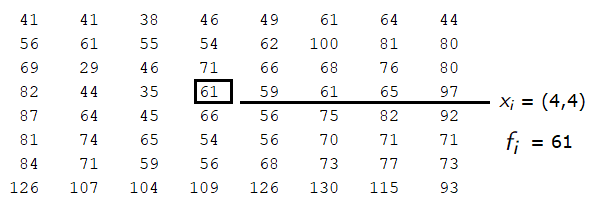
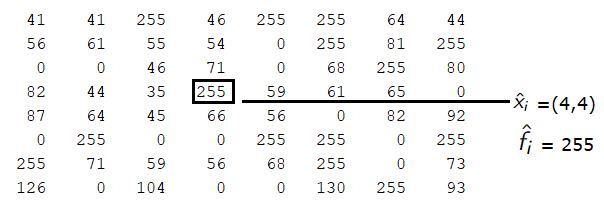
Consider an original, uncorrupted black-and-white image whose matrix representation is denoted by , where each entry stores a pixel value of the image. Sometimes the image may contain defective pixels, which can be restored based on the correct pixel values that are available. Let us denote the matrix representation of the corrupted image by . The coordinates of a valid pixel are denoted by , i.e., and the coordinates of a defective pixel are , i.e., . Given the fact that the correct pixels are known, the goal is to reconstruct the values for all . In our approach, we are going to deliberately corrupt several pixels using the Salt-and-Pepper noise. This consists of changing the values of a specific percentage of pixels into (black = pepper) or (white = salt), as in
| (5) |
Figure 1 shows the matrix form of a black-and-white image with resolution in both cases: as an uncorrupted image (Subfigure 1(a)) and as a corrupted image using the Salt-and-Pepper noise for of the pixels (Subfigure 1(b)).
III-A Global case
Paewpolsong et al. [Pae22] proposed an algorithm to reconstruct images that were damaged by Salt-and-Pepper noise. Their reconstruction method is based on using shapefree radial basis functions neural networks. Following some ideas proposed in this paper, we consider the reconstruction of a damaged black-and-white image using the bivariate Shepard operator introduced in (1). For the reconstruction, we will use a global approach, where the value of a defective pixel is computed based on all the information provided by the set of correct pixels. Consider the matrix associated with an image of resolution that contains a percentage of damaged pixels. Let be the number of valid pixels and be the number of defective pixels.
Let be the set of interpolation nodes, where and represent the matrix coordinates of the correct pixels , . We apply the Shepard operator given in (1) to reconstruct the set of defective pixels, . The reconstructed values of the damaged pixels are obtained as The new matrix corresponding to the reconstructed image will have the form:
The pseudo-code for this approach is given in Algorithm 1.
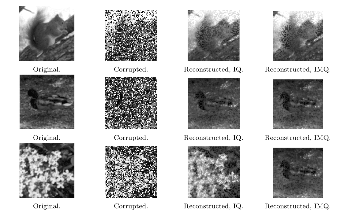
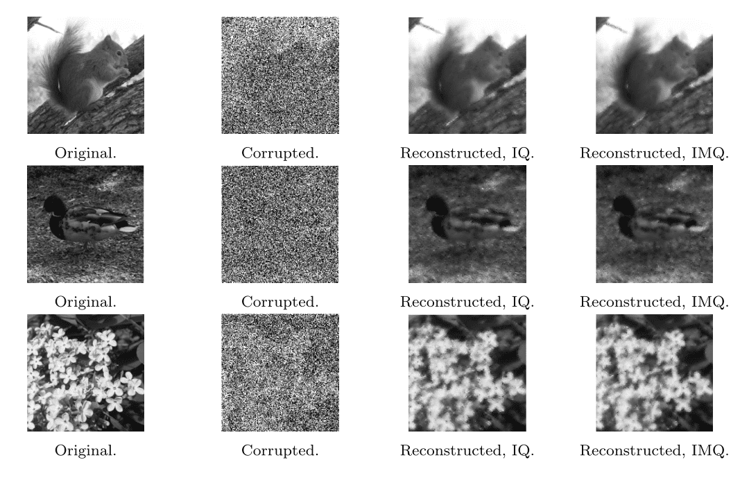
For numerical experiments we considered three images downloaded from the TAMPERE17 noise-free image database \urlhttps://webpages.tuni.fi/imaging/tampere17/ with a resolution of pixels. We corrupted of the pixels with the Salt-and-Pepper noise and reconstructed them using the Shepard operator (1) combined with both RBFs, inverse quadratic (IQ) () and inverse multiquadric (IMQ) (). The experiments were performed in Matlab, and the results are shown in Figure 2.
III-B Local case
In the global method, an incorrect pixel’s value is reconstructed based on all the information provided by the correct pixels. However, this approach does not always produce the best results for the reconstructed image, since the pixels of an image have strongly local properties, as emphasized in [Ska13]. It may be more efficient to approximate the value of an incorrect pixel based on a local procedure. In [UhSka05], the focus was on reconstructing black-and-white images using the radial basis function approach in some neighborhoods of the defective pixels. The neighborhood is defined by a radius that moves in both directions of the axes and , creating a window of dimensions (see, e.g., [ZapVanSka08]).
The radius size could be chosen according to the image that is processed, but its choice is not an easy task. In Figure 3, a pixel’s neighborhood of radius is represented.
This approach leads to a smaller computational time compared to the global case, especially for high-resolution images because the systems (4) have a significantly reduced size.
The reconstruction of the damaged pixels is based on the combined Shepard operator given in (1) used locally, in each neighborhood. Besides the local behavior, some other differences appear in the algorithm, in contrast to the global case. First, a pixel is reconstructed only if a certain percentage of correct pixel exists within its neighborhood, determined by an initial desired tolerance . If this condition is not met, the value is not restored, the algorithm continues and the procedure is retried in the next iteration. The shape parameter of the functions defined in (3) is updated at each iteration based on the new set of correct pixels that is constructed. Finally, to avoid the case when the algorithm gets stuck due to the impossibility of reconstructing new pixels because of the unattained criteria, the tolerance can be increased after each iteration. This adjustment allows the reconstruction of a pixel even if the initial desired number of correct pixels in its neighborhood was not achieved. The pseudo-code is presented in Algorithm 2.
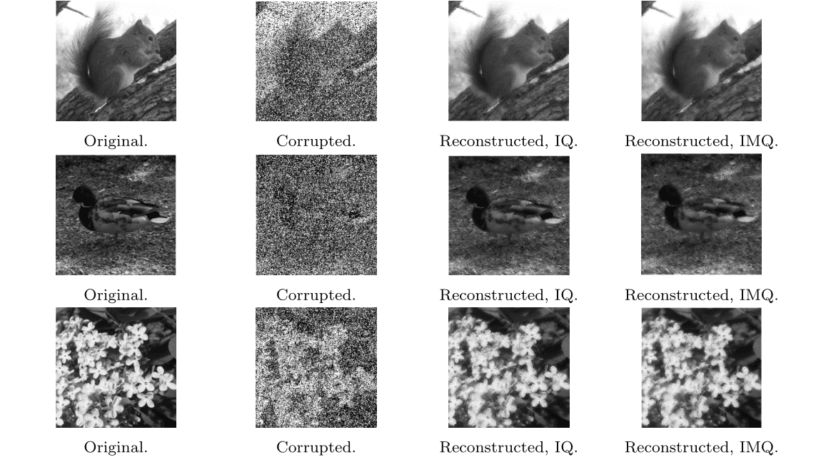
For the numerical experiments in this case, we used the previously mentioned images, considering three different resolutions: , , and pixels, respectively. The pixels corrupted with the Salt-and-Pepper noise were reconstructed using the Shepard operators (1) combined with the inverse quadratic (IQ) () and inverse multiquadric (IMQ) () radial basis functions. The radius of the neighborhood considered was , and the initial tolerance was set to . We computed the Mean Absolute Errors (MAEs) and the Mean Square Errors (MSEs), defined as
| (6) | ||||
| (7) |
where is the resolution of the image, is the matrix corresponding to the original image (without the damaged pixels), is the reconstructed image, and is the number of all the pixels ( and the number of all the damaged pixels (), respectively. Table I presents the numerical results obtained in the case of defective pixels. The graphical representations for the case of pixels resolution are shown in Figure 4(a). Table II presents the MAEs and MSEs for the case of 75 defective pixels. The graphical representations in the case of pixels are shown in Figure 4(b). In both cases, we compared the results with the ones obtained using the classical Shepard operator for image restoration (SC). It is defined as
| (8) |
for some known values of a target function to be reconstructed on a set of sample points with given in (2), considering . Moreover, we performed the same tests using the radial basis function method as a reconstruction technique, as proposed, for example, in [UhSka05]. We considered the same RBFs used for the Shepard method: the inverse quadratic (RBF-IQ) and the inverse multiquadric (RBF-IMQ). We can observe that the results are comparable, emphasizing that the choice of the operator used depends on the available data sets. All the computations were performed in Matlab.
| Image | Size | IQ | IMQ | RBF-IQ | RBF-IMQ | SC | ||||||
|---|---|---|---|---|---|---|---|---|---|---|---|---|
| (pixels) | ||||||||||||
| 64 | MAE | 3.0488 | 6.4537 | 3.8503 | 7.7881 | 3.8838 | 7.9580 | 1.9785 | 4.0765 | 4.0989 | 7.5126 | |
| MSE | 29.2734 | 61.9659 | 35.3613 | 71.2664 | 34.9431 | 71.5993 | 17.4766 | 36.0080 | 36.1318 | 67.0200 | ||
| Squirrel | 128 | MAE | 2.6635 | 5.4466 | 2.7916 | 5.8035 | 3.0629 | 6.3066 | 2.6510 | 5.4130 | 2.9958 | 5.5836 |
| MSE | 24.8775 | 50.8728 | 25.2861 | 52.5679 | 27.7273 | 57.0924 | 24.2982 | 49.6138 | 25.5072 | 52.2310 | ||
| 256 | MAE | 2.0421 | 4.2144 | 2.3256 | 4.7664 | 1.3852 | 2.8604 | 2.7158 | 5.3699 | 2.6661 | 4.4314 | |
| MSE | 19.1413 | 39.5037 | 21.5356 | 44.1379 | 12.4294 | 25.6664 | 25.6967 | 50.8104 | 19.4090 | 41.7361 | ||
| 64 | MAE | 3.3040 | 6.6144 | 3.6333 | 7.2524 | 4.3599 | 8.6146 | 3.6831 | 7.2739 | 3.4768 | 5.9488 | |
| MSE | 34.0203 | 68.1070 | 36.5508 | 72.9591 | 42.5686 | 84.1105 | 37.0300 | 73.1316 | 34.6287 | 59.2093 | ||
| Duck | 128 | MAE | 3.7920 | 7.6654 | 3.9347 | 7.8752 | 4.4873 | 8.8782 | 2.9347 | 5.9141 | 3.3517 | 6.6608 |
| MSE | 37.4204 | 75.6442 | 38.4586 | 76.9736 | 42.2457 | 83.5833 | 28.6941 | 57.8258 | 32.4424 | 74.4776 | ||
| 256 | MAE | 2.8885 | 6.7603 | 3.3504 | 7.7502 | 2.9630 | 5.9133 | 4.0513 | 8.1227 | 2.7705 | 5.5314 | |
| MSE | 30.3921 | 62.6268 | 30.3486 | 62.1441 | 28.1477 | 56.1738 | 37.3027 | 74.7903 | 24.5686 | 49.0519 | ||
| 64 | MAE | 7.8159 | 15.7317 | 8.6021 | 17.1873 | 5.5688 | 11.2921 | 8.7522 | 17.3100 | 7.2290 | 14.2836 | |
| MSE | 52.0884 | 104.8422 | 52.8828 | 105.6624 | 42.6194 | 86.4203 | 55.7437 | 110.2492 | 47.0215 | 92.9088 | ||
| Lilac | 128 | MAE | 6.4549 | 12.9971 | 7.3460 | 14.6562 | 7.5515 | 15.2032 | 3.2698 | 6.5605 | 5.6881 | 11.3499 |
| MSE | 45.0393 | 90.6875 | 46. 7339 | 93.2403 | 46.9867 | 94.5970 | 27.0303 | 54.2327 | 39.1420 | 78.1028 | ||
| 256 | MAE | 4.5035 | 9.0432 | 5.1046 | 10.1667 | 5.1958 | 10.4333 | 4.3784 | 8.7962 | 3.4615 | 6.9085 | |
| MSE | 34.7859 | 69.6511 | 37.3420 | 74.3730 | 37.3673 | 75.0345 | 33.6234 | 67.5497 | 26.8552 | 53.5976 | ||
| Image | Size | IQ | IMQ | RBF-IQ | RBF-IMQ | SC | ||||||
|---|---|---|---|---|---|---|---|---|---|---|---|---|
| (pixels) | ||||||||||||
| 64 | MAE | 5.7886 | 7.9165 | 6.1357 | 8.3941 | 6.6062 | 9.0771 | 3.8699 | 5.3370 | 9.1814 | 12.6623 | |
| MSE | 52.8901 | 72.3332 | 54.7422 | 74.8911 | 57.0402 | 78.3753 | 35.1724 | 48.5071 | 71.0435 | 97.9778 | ||
| Squirrel | 128 | MAE | 4.5025 | 6.1633 | 4.6560 | 6.3485 | 4.5613 | 6.2387 | 3.0633 | 4.1810 | 5.9568 | 8.1412 |
| MSE | 41.3348 | 56.5820 | 42.4871 | 57.9318 | 40.3003 | 55.1198 | 27.3839 | 37.3757 | 48.6407 | 66.4772 | ||
| 256 | MAE | 3.5675 | 4.8870 | 3.7372 | 5.1113 | 3.6951 | 5.0583 | 3.4109 | 4.6693 | 4.9520 | 6.6118 | |
| MSE | 32.8042 | 44.9376 | 34.3066 | 46.9211 | 33.8474 | 46.3345 | 31.5244 | 43.1546 | 46.2881 | 61.3837 | ||
| 64 | MAE | 5.8584 | 7.7833 | 5.3125 | 6.9543 | 7.0669 | 9.3465 | 5.4187 | 7.2485 | 5.6411 | 7.2084 | |
| MSE | 64.2800 | 85.0149 | 65.9153 | 87.1776 | 66.4197 | 87.8447 | 53.3684 | 71.3903 | 55.8879 | 71.3837 | ||
| Duck | 128 | MAE | 6.3166 | 8.4290 | 6.5463 | 8.7577 | 6.3074 | 8.3798 | 6.3390 | 8.4990 | 5.3077 | 7.0592 |
| MSE | 60.6191 | 80.8913 | 61.3469 | 82.0697 | 60.1147 | 79.8670 | 60.4590 | 81.0606 | 48.8678 | 64.9931 | ||
| 256 | MAE | 5.5304 | 7.6872 | 5.6804 | 7.8754 | 5.3715 | 7.1759 | 6.5068 | 8.6925 | 5.0627 | 6.7633 | |
| MSE | 49.2334 | 58.7967 | 49.7614 | 59.3976 | 49.5005 | 66.1285 | 58.4281 | 78.0550 | 43.7449 | 58.4395 | ||
| 64 | MAE | 13.9375 | 18.5290 | 14.3804 | 19.1178 | 10.8867 | 14.4732 | 9.8218 | 13.1042 | 15.0703 | 19.7726 | |
| MSE | 84.0781 | 111.7767 | 85.8694 | 114.1581 | 74.5144 | 99.0623 | 65.7292 | 87.6961 | 80.7622 | 113.7531 | ||
| Lilac | 128 | MAE | 11.1888 | 15.0015 | 10.3228 | 14.4397 | 11.9753 | 16.0100 | 10.8036 | 14.4827 | 11.1688 | 14.9257 |
| MSE | 71.2964 | 95.5908 | 71.1661 | 95.1823 | 74.6075 | 99.7446 | 69.7742 | 93.5346 | 77.6111 | 99.3511 | ||
| 256 | MAE | 7.9741 | 10.6209 | 7.1637 | 9.8769 | 5.0419 | 6.7100 | 7.4306 | 9.9266 | 8.2623 | 10.6803 | |
| MSE | 57.1398 | 76.1058 | 55.4276 | 77.8465 | 40.9014 | 54.4333 | 54.5833 | 72.9187 | 56.1876 | 78.8978 | ||
IV Reconstruction of damaged color images using the bivariate multivalued Shepard operator
Consider a multivalued function , and a set of interpolation nodes . The Shepard-type multivalued interpolation operator was defined in [SomSoos16] as
| (9) |
for , given in (2), . Based on this, we can define the multivalued Shepard operator combined with inverse quadratic and inverse multiquadric RBF in the bivariate case as
| (10) |
for , given in (2), , and
| (11) |
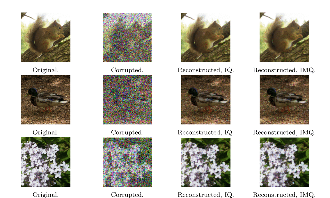
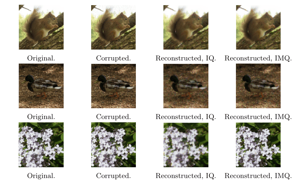
The coefficients are found solving similar systems as the one in (4). A color image is represented as an structure with each component defining the colors red, green, and blue (RGB) of every pixel. To reconstruct colored images, we use the multivalued Shepard operator introduced in (10) for , applying similar methods as for black-and-white images. Computationally, we apply Algorithm 2 to each of the three color components: red, green, and blue. We consider only the case of local approximation and since the reconstructions of the three components are independent, we consider parallel computing, performed in Matlab. For numerical examples, we corrupted 50 of the pixels using the Salt-and-Pepper noise. We used the multivalued Shepard operator given in (10) for (IQ) and (IMQ) to reconstruct the previously mentioned images in color format. The images were processed with a resolution of pixels (Figure 5), using neighborhoods of radius and an initial tolerance . The shape parameter was computed following the previously mentioned ideas (see, e.g., [Har71]).
V Reconstruction of images damaged with Gaussian and Poisson noises
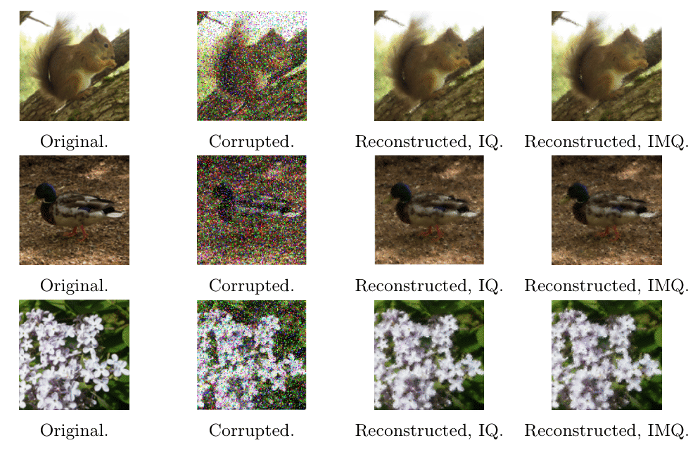
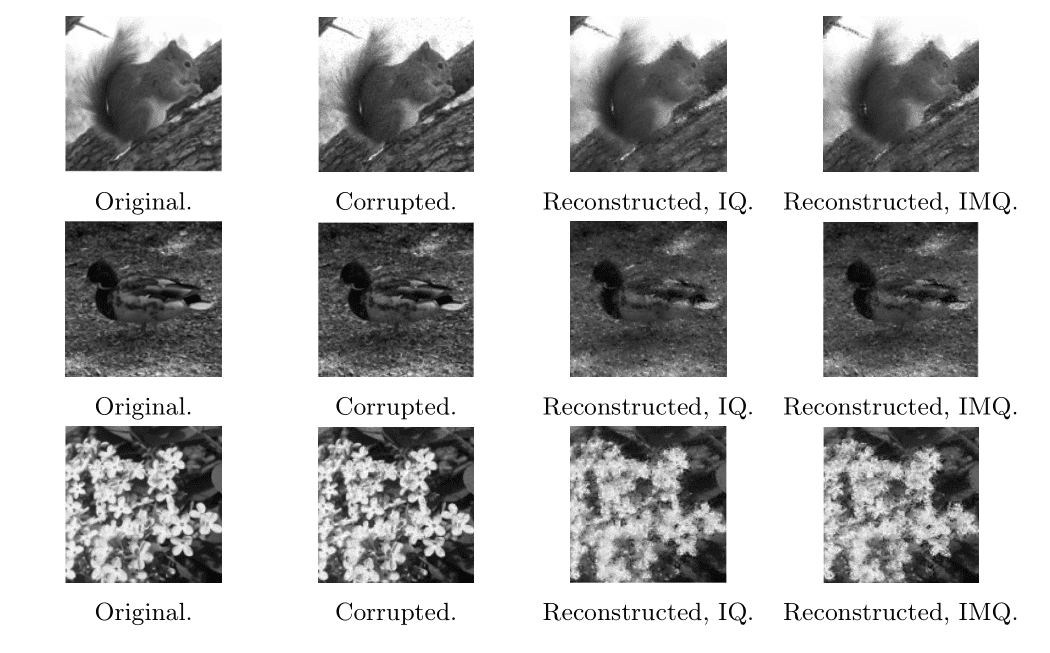
In the last part of this paper, we consider two additional types of noise, specifically Gaussian and Poisson noise, applied to corrupt of the pixels in the previously mentioned images. We consider a resolution of pixels, for both black-and-white and color images.
For Gaussian noise, the corrupted pixels are obtained as , where represents noise sampled from a Gaussian distribution. The visual representations are shown in Figure 6.

Poisson noise, rather than being added artificially, is generated from the data following a Poisson distribution. The graphical representations for this case are shown in Figure 7.
It can be observed that this operator is effective in reconstructing various types of damaged images. A more in-depth study of the latter two types of noise could be a subject for future research.
VI Conclusions
In this paper, we focused on the restoration of black-and-white and color images. The Shepard operator is well-known for its advantages in reconstructing function values from a limited number of known data points, and its practical benefits in image reconstruction have been demonstrated through the methods discussed above. We proposed two approaches: a global and a local one, with the latter providing better results, as expected.
[1] R. Caira, F. Dell’Accio, and F. Di Tommaso. “On the bivariate Shepard–Lidstone operators”. In: J. Comput. Appl. Math. 236 (2012), pp. 1691–1707.
[2] T. Cătinaș. “The bivariate Shepard operator of Bernoulli type”. In: Calcolo 44.4 (2007), pp. 189–202.
[3] T. Cătinaș. “The combined Shepard-Lidstone bivariate operator”. In: Trends and Applications in Constructive Approximation. Ed. by D.H. Mache, J. Szabados, and M.G. de Bruin. Vol. 151. Basel: Birkhauser Basel, 2005, pp. 77–89.
[4] T. Cătinaș and A. Malina. “Shepard operator of least squares thin-plate spline type”. In: Stud. Univ. Babeș-Bolyai Math. 66 (2021), pp. 257–265.
[5] T. Cătinaș and A. Malina. “The combined Shepard operator of inverse quadratic and inverse multiquadric type”. In: Stud. Univ. Babeș-Bolyai Math. 67 (2022), pp. 579–589.
[6] F. Dell’Accio and F. Di Tommaso. “Complete Hermite–Birkhoff interpolation on scattered data by combined Shepard operators”. In: J. Comput. Appl. Math. 300 (2016), pp. 192–206.
[7] G.E. Fasshauer and J.G. Zhang. “On choosing “optimal” shape parameters for RBF approximation”. In: Numer. Algor. 45 (2007), pp. 345–368.
[8] R. Franke. “Scattered data interpolation: tests of some methods”. In: Math. Comp. 385 (1982), pp. 181–200.
[9] R. Franke and G. Nielson. “Smooth interpolation of large sets of scattered data”. In: Int. J. Numer. Meths. Engrg. 15 (1980), pp. 1691–1704.
[10] R. Hardy. “Multiquadric equations of topography and other irregular surfaces”. In: J. Geophys. Res. 76 (1971), pp. 1905–1915.
[11] P. Paewpolsong et al. “Image reconstruction by shape-free radial basis function neural networks (RBFNs)”. In: Journal of Physics: Conference Series 2312.1 (2022).
[12] J. Ren et al. “Shepard Convolutional Neural Networks”. In: Advances in Neural Information Processing Systems. Vol. 28. Curran Associates, Inc., 2015.
[13] R.J. Renka. “Algorithm 790: CSHEP2D: Cubic method for bivariate interpolation of scattered data”. In: ACM Trans. Math. Software 25 (1999), pp. 70–73.
[14] R.J. Renka. “Multivariate interpolation of large sets of scattered data”. In: ACM Trans. Math. Software 14 (1988), pp. 139–148.
[15] V. Savchenko, N. Kojekine, and H. Unno. “A practical image retouching method”. In: CW ’02: Proceedings of the First International Symposium on Cyber Worlds. 2002, pp. 480–487.
[16] D. Shepard. “A two dimensional interpolation function for irregularly spaced data”. In: Proceedings of the 1968.
[17] V. Skala. “Fast Reconstruction of Corrupted Images and Videos by Radial Basis Functions”. In: ICCAIS 2013 Conf. 2013, pp. 267–271.
[18] K. Smith and P. Williams. “Time Series Classification with Shallow Learning Shepard Interpolation Neural Networks”. In: Image and Signal Processing. Springer International Publishing, 2018, pp. 329–338.
[19] K. Smith et al. “Deep Convolutional-Shepard Interpolation Neural Networks for Image Classification Tasks”. In: Image Analysis and Recognition. Springer International Publishing, 2018, pp. 185–192.
[20] K. Smith et al. “Shepard Interpolation Neural Networks with K-Means: A Shallow Learning Method for Time Series Classification”. In: 2018 International Joint Conference on Neural Networks (IJCNN). 2018, pp. 1–6.
[21] I. Somogyi and A. Soos. “Interpolation methods for multivalued functions”. In: Stud. Univ. Babeș-Bolyai Math. 61 (2016), pp. 377–382.
[22] K. Uhlir and V. Skala. “Reconstruction of damaged images using Radial Basis Functions”. In: 2005 13th European Signal Processing Conference. 2005, pp. 1–4.
[23] P. Wen, X. Wu, and C. Wu. “An interactive image inpainting method based on RBF networks”. In: Advances in Neural Networks 3972 (2006), pp. 629–637.
[24] P. Williams. “SINN: Shepard Interpolation Neural Networks”. In: Advances in Visual Computing. Springer International Publishing, 2016, pp. 349–358.
[25] J. Zapletal, P. Vanecek, and V. Skala. “Influence of essential parameters on the RBF based image reconstruction”. In: Proceedings of SCCG 2008. 2008, pp. 178–185.
[26] J. Zapletal, P. Vanecek, and V. Skala. “RBF-based image restoration utilising auxiliary points”. In: Computer Graphics International Conference, ACM. 2009, pp. 39–44.