Posts by Maria Crăciun

Abstract

The purpose of the article is to highlight the role of binomial polynomials in the construction of classes of positive linear approximation sequences on Banach spaces. Our results aim to introduce and study an integral extension in Kantorovich sense of these binomial operators, which are useful in approximating signals in $L_{p} ([0, 1])$ spaces, $p \geq 1$ . Also, inspired by the coincidence index that appears in the definition of entropy, a general class of discrete operators related to the squared fundamental basis functions is under study. The fundamental tools used in error evaluation are the smoothness moduli and Peetre’s K-functionals. In a distinct section, numerical applications are presented and analyzed.

Authors

Octavian Agratini
Tiberiu Popoviciu’ Institute of Numerical Analysis, Romanian Academy, Cluj-Napoca, Romania

Maria Crăciun
Tiberiu Popoviciu’ Institute of Numerical Analysis, Romanian Academy, Cluj-Napoca, Romania

Keywords

binomial polynomial; umbral calculus; linear positive operator; r-modulus of smoothness; Peetre’s K-functionals; Kantorovich-type operator; Hardy–Littlewood maximal operator; index of coincidence

Paper coordinates

O. Agratini, M. Crăciun, Linear approximation processes based on binomial polynomials. Mathematics. 2025; 13(15):2413. https://doi.org/10.3390/math13152413

PDF

https://ictp.acad.ro/wp-content/uploads/2025/09/2025-Agratini-Craciun-Linear.pdf

Journal: www.mdpi.com/2227-7390/13/15/2413

About this paper

Journal

Mathematics

Publisher Name

MDPI

DOI

https://doi.org/10.3390/math13152413

Print ISSN

Online ISSN

2227-7390

google scholar link

Preprint in HTML form

Linear Approximation Processes Based on Binomial Polynomials

Octavian Agratini and Maria Crăciun

Tiberiu Popoviciu Institute of Numerical Analysis,
Romanian Academy,
P.O. Box 68-1, 400110 Cluj-Napoca, Romania

Abstract

The purpose of the article is to highlight the role of binomial polynomials in the construction of classes of positive linear approximation sequences on Banach spaces. Our results aim to introduce and study an integral extension in Kantorovich sense of these binomial operators, which are useful in approximating signals in $L_{p}([0,1])$ spaces, $p\geq 1$ . Also, inspired by the coincidence index that appears in the definition of entropy, a general class of discrete operators related to the squared fundamental basis functions is under study. The fundamental tools used in error evaluation are the smoothness moduli and Peetre’s K-functionals. In a distinct section, numerical applications are presented and analyzed.

Keywords: binomial polynomial; umbral calculus; linear positive operator; r-modulus of smoothness; Peetre’s K-functionals; Kantorovich-type operator; Hardy–Littlewood maximal operator;index of coincidence

MSC 41A36; 41A25

1 Introduction

The roots of this paper are based on binomial polynomials, which have their origin in the so-called Heaviside calculus created by G. Boole. We point out that the first rigorous version of this calculus belongs to Gian-Carlo Rota and his collaborators, see for example, [1, 2]. To achieve a self-contained exposition, we will recall the notions of a polynomial sequence of binomial type and some facts needed in the subsequent analysis accompanied by several examples. Thus, we arrive at the main part of the paper: applications of the binomial sequences in the construction of linear approximation processes. In particular cases, some classical operators are highlighted. We will examine new extensions of these operators, both integral in the Kantorovich sense and connected with squared fundamental functions, proving approximation properties of the new constructions.

We mention the role of binomial polynomials in Approximation Theory by exploiting the technique of the umbral calculus or symbolic calculus. This calculus is a successful combination of the differences among calculus and certain chapters of Functional Analysis and Probability Theory. We emphasize that this kind of study is still in the spotlight of many papers. Through the integral constructions presented in the manuscript, we manage to approximate functions from larger normed spaces. In other recent works, various methods were employed to solve linear and nonlinear differential equations with the help of bases generated by some specific polynomials.

Considering $I\subset\mathbb{R}$ an interval, we work in different spaces: $C(I)$ the space of continuous real-valued functions defined on $I$ , $L_{p}(I)$ the space of all $p$ -th power integrable functions on $I$ $(1\leq p<\infty)$ . The main tools used are the r-modulus of smoothness, K-functional, and Hardy–Littlewood maximal operator. In a separate section, the theoretical aspects are complemented by numerical examples that confirm our results.

2 Preliminaries

Set $\mathbb{N}_{0}=\{0\}\cup\mathbb{N}$ . For any $n\in\mathbb{N}_{0}$ , we denote by $\Pi_{n}$ the linear space of polynomials of degree no greater than $n$ and by $\Pi_{n}^{*}$ the set of all polynomials of degree $n$ . In our study, we only consider polynomials with real coefficients. We set

\Pi:=\bigcup_{n\geq 0}\Pi_{n}.

which represents the commutative algebra of polynomials with coefficients on the field $\mathbb{R}$ .

A sequence $p=(p_{n})_{n\geq 0}$ such that $p_{n}\in\Pi_{n}^{*}$ for every $n\in\mathbb{N}_{0}$ is called a polynomial sequence.

Definition 1.

A polynomial sequence $b=(b_{n})_{n\geq 0}$ is of binomial type if for any $(x,y)\in\mathbb{R}\times\mathbb{R}$ the following equality

b_{n}(x+y)=\sum_{k=0}^{n}\displaystyle\binom{n}{k}b_{k}(x)b_{n-k}(y),\quad n% \in\mathbb{N}_{0},\vskip-6.0pt

(1)

holds.

Remark 1.

Knowing that $\deg(b_{0})=0$ , we obtain $b_{0}(x)=1$ for any $x\in\mathbb{R}$ and by induction we obtain $b_{n}(0)=0$ for any $n\in\mathbb{N}$ .

The trivial example of the binomial sequence is $e=(e_{n})_{n\geq 0}$ , $e_{n}(x)=x^{n}$ . Some nontrivial examples are given below:

(i) The generalized factorial power with step $a$ :

$p=(p_{n})_{n\geq 0}$ ,

p_{0}(x)=x^{[0,x]}:=1\mbox{ and }p_{n}(x)=x^{[n,a]}:=x(x-a)\ldots(x-(n-1)a),% \quad n\in\mathbb{N}.

Particular cases: for $a=-1$ , we obtain the lower-factorials denoted by $\langle x\rangle_{n}$ ; for $a=1$ , we obtain the upper-factorials denoted by $(x)_{n}$ .

(ii) Touchard polynomials: $t=(t_{n})_{n\geq 0}$ ,

t_{n}(x)=\sum_{k=0}^{n}S(n,k)x^{k},

where $S(n,k)$ represent the Stirling numbers of the second kind defined by

x^{n}=\sum_{k=0}^{n}S(n,k)\langle x\rangle_{k}.\vskip-6.0pt

The Dobinski formula says

t_{n}(x)=e^{-x}\sum_{k=0}^{\infty}\displaystyle\frac{k^{n}}{k!}x^{k},

see [1].

(iii) Abel polynomials: $\widetilde{a}=(a_{n}^{\langle a\rangle})_{n\geq 0},\quad a\neq 0$ ,

a_{0}^{\langle a\rangle}=1,\quad a_{n}^{\langle a\rangle}(x)=x(x-na)^{n-1},% \quad n\in\mathbb{N}.

(iv) Gould polynomials: $g=(g_{n}^{(a,b)})_{n\geq 0},\quad ab\neq 0$ ,

g_{0}^{(a,b)}=1,\quad g_{n}^{(a,b)}(x)=\displaystyle\frac{x}{x-an}\left\langle% \displaystyle\frac{x-an}{b}\right\rangle_{n},\quad n\in\mathbb{N}.

In what follows, set $\mathcal{L}$ as the space of all linear operators $T:\Pi\to\Pi$ . For a given $a\in\mathbb{R}$ , $E^{a}\in\mathcal{L}$ stands for the shift operator defined by the relation

(E^{a}p)(x)=p(x+a),\quad p\in\Pi.

Definition 2.

An operator $T\in\mathcal{L}$ , which is switched with all shift operators, that is $TE^{a}=E^{a}T$ , $a\in\mathbb{R}$ , is called a shift-invariant operator.

The class of these operators is denoted by $\mathcal{L}_{s}$ .

Definition 3.

An operator $Q$ is called a delta operator if $Q\in\mathcal{L}_{s}$ and $Qe_{1}$ is a nonzero constant.

Let $\mathcal{L}_{\delta}$ denote the set of all delta operators.

According to [2] (Proposition 2), for every $Q\in\mathcal{L}_{\delta}$ , we have

Q(\Pi_{n}^{*})\subset Q(\Pi_{n-1}^{*}),\quad n\in\mathbb{N}.

We present some well-known examples of delta operators. Here, $I$ stands for the identity operator on the space $\Pi$ .

(i) The derivative operator, denoted by $D$ .

(ii) The operators used in calculus with divided differences. Let $h\in\mathbb{R}$ be a fixed number. We set

\Delta_{h}:=E^{h}-I,\quad\nabla_{h}:=I-E^{-h},\quad\delta_{h}:=E^{h/2}-E^{-h/2},

representing the forward difference, the backward difference, and the central difference operator, respectively.

(iii) Abel operator $A_{a}=DE^{a}$ , $a\neq 0$ . For any $p\in\Pi$ ,

(A_{a}p)(x)=\displaystyle\frac{dp}{dx}(x+a).

Writing Taylor’s series in the following manner

E^{a}=\sum_{\nu=0}^{\infty}\displaystyle\frac{h^{\nu}D^{\nu}}{\nu!}=e^{hD},

we can also get $A_{a}=D(e^{aD})$ .

(iv) Touchard operator

T:=\log(I+D)=D-\displaystyle\frac{D^{2}}{2}+\displaystyle\frac{D^{3}}{3}-\ldots,

for any polynomial, with the sum being finite.

Another representation of this operator is based on divided differences as follows

(T_{p})(x)=\int_{0}^{\infty}e^{-t}[x,x-t;p]dt,\quad p\in\Pi.

(v) Gould operator, $G_{a,b}:=\Delta_{b}E^{a}=E^{a+b}E^{a}$ , $ab\neq 0$ .

Definition 4.

Let $Q$ be a delta operator. A polynomial sequence $p=(p_{n})_{n\geq 0}$ is called the sequence of basic polynomials associated with $Q$ if

(i) $p_{0}(x)=1$ for any $x\in\mathbb{R}$ ;

(ii) $p_{n}(0)=0$ for any $n\in\mathbb{N}$ ;

(iii) $(Qp_{n})(x)=np_{n-1}(x)$ for any $(n,x)\in\mathbb{N}\times\mathbb{R}$ .

Remark 2.

If $p=(p_{n})_{n\geq 0}$ is a sequence of basic polynomials associated with $Q\in\mathcal{L}_{\delta}$ , then $\{p_{0},p_{1},\ldots,p_{n-1},e_{n}\}$ is a basis of the vectorial space $\Pi_{n}$ . Taking this fact into account, by induction, it can be proved [2] (Proposition 3) that every delta operator has a unique sequence of basic polynomials.

For example, $(e_{n})_{n\geq 0}$ , $(x^{[n,h]})_{n\geq 0}$ , and $(x+(n-1)h)_{n\geq 0}^{[n,h]}$ represent the sequence of basic polynomials associated with $Q=D$ , $Q=\Delta_{h}$ , and $Q=\nabla_{h}$ , respectively. Also, $\widetilde{a}=(a_{n}^{\langle a\rangle})_{n\geq 0}$ and $g=(g_{n}^{(a,b)})_{n\geq 0}$ are the sequence of basic polynomials associated with the Abel operator $A_{a}$ and Gould operator $G_{a,b}$ .

We conclude this paragraph by presenting the connection between the delta operator and the binomial type sequences.

Theorem 1 ([2], Theorem 1).

(a) If $p=(p_{n})_{n\geq 0}$ is a basic sequence for some delta operator $Q$ , then it is a sequence of binomial type.

(b) If $p=(p_{n})_{n\geq 0}$ is a sequence of binomial type, then it is a basic sequence for some delta operator.

3 Operators of Binomial Type

We consider a delta operator $Q$ and its sequence of basic polynomials $p=(p_{n})_{n\geq 0}$ . For every $n\geq 1$ , we consider the operator $L_{n}^{Q}:C([0,1])\to C([0,1])$ defined as follows

(L_{n}^{Q}f)(x)=\displaystyle\frac{1}{p_{n}(1)}\sum_{k=0}^{n}\displaystyle% \binom{n}{k}p_{k}(x)p_{n-k}(1-x)f\left(\displaystyle\frac{k}{n}\right),\quad n% \in\mathbb{N}.\vskip-6.0pt

(2)

According to Sablonierre [3], they are called Bernstein–Sheffer operators , but as Stancu and Occorsio stated [4], these operators can be named Popoviciu operators because, in fact, they were first defined in a note published by T. Popoviciu [5].

Remark 3.

Since any compact interval is isomorphic to $[0,1]$ , the use of this compact interval does not restrict the usefulness of the operators.

The operators $L_{n}^{Q}$ , $n\in\mathbb{N}$ , are linear and reproduce the constants. Indeed, choosing $y:=1-x$ in (1), we obtain $L_{n}^{Q}e_{0}=e_{0}$ . Moreover, these operators interpolate functions at the ends of their domain.

The positivity of these operators is given by the sign of the coefficients of the series $\varphi(t)=c_{1}+c_{2}t+\ldots$ $(c_{1}\neq 0)$ . More precisely, Popoviciu [5], and later Sablonniere [3] (Theorem 1),

have established

Lemma 1.

$L_{n}^{Q}$ is a positive operator on $C([0,1])$ for every $n\geq 1$ if and only if $c_{1}>0$ and $c_{n}\geq 0$ for all $n\geq 2$ .

We specify that the above series $\varphi$ is connected with a sequence of basic polynomials $(p_{n})_{n\geq 0}$ by the relation

e^{x\varphi(t)}=\sum_{n\geq 0}\displaystyle\frac{p_{n}(x)}{n!}t^{n},

see [2] (Corollary 3). In what follows, we point out significant results of the operators defined by (2), see, e.g., [3] (Theorems 2 and 3).

Theorem 2.

If the operators $L_{n}^{Q}$ , $n\geq 1$ , defined by (2) satisfy the conditions of Lemma 1, then the following statements are true:

(i) $L_{n}^{Q}$ is an isomorphism of $\Pi_{n}$ preserving the degree, i.e., $L_{n}^{Q}q\in\Pi_{k}$ whenever $q\in\Pi_{k}$ , $0\leq k\leq n$ .

(ii) The behavior of operators on Korovkin test functions is as follows

L_{n}^{Q}e_{j}=e_{j},\quad j\in\{0,1\},\quad n\in\mathbb{N},\vskip-6.0pt

(3)

L_{n}^{Q}e_{2}=e_{2}+a_{n}(e_{1}-e_{2}),\quad n\geq 2,

(4)

where $a_{n}=\displaystyle\frac{1}{n}\left(1+(n-1)\displaystyle\frac{r_{n-2}(1)}{p_{n% }(1)}\right)$ , the sequence $(r_{n}(x))_{n\geq 0}$ being generated by

\varphi^{\prime\prime}(t)\exp(x\varphi(t))=\sum_{n\geq 0}r_{n}(x)\displaystyle% \frac{t^{n}}{n!}.

(5)

(iii) $L_{n}^{Q}$ converges uniformly to $f\in C([0,1])$ if and only if the condition

\lim\limits_{n\to\infty}(r_{n-2}(1)/p_{n}(1))=0\vskip-6.0pt

(6)

holds.

(iv) If

r_{n-2}(1)/p_{n}(1)=\mathcal{O}\left(\displaystyle\frac{1}{n}\right),

(7)

then there exists an integer $k\geq 1$ for which $\varphi\in\Pi_{k}$ , and we have

\|L_{n}^{Q}f-f\|_{\infty}\leq\left(1+\sqrt{k}/2\right)\omega_{1}\left(f;1/% \sqrt{n}\right).

In the above, $\|\cdot\|_{\infty}$ is the sup-norm of the Banach space $C([0,1])$ , and $\omega_{1}(f;\cdot)$ is the first modulus of continuity of $f$ . We recall

\omega_{1}(f;\delta):=\sup\{|f(x)-f(y)|:\ x,y\in[0,1],\ |x-y|\leq\delta\},% \quad\delta\geq 0.\vskip-6.0pt

(8)

We specify that relations (3) imply that the operators reproduce affine functions; consequently, they are of Markov type.

Remark 4.

Choosing certain particular cases of delta operators in (2) already presented in the previous section, we reobtain some classical linear positive operators of a discrete type.

(i) In the case $Q=D$ , we obtain the well-known Bernstein operators. In this case, (4) becomes $L_{n}^{D}e_{2}=e_{2}+(e_{1}-e_{2})/n.$

Statement (iv) of Theorem 2 shows that the Bernstein operators $L_{n}^{D}$ $(k=1)$ , could be considered as the best positive operators of binomial type associated with any function $\varphi\in\Pi_{n}$ .

(ii) If $Q=\displaystyle\frac{1}{\alpha}\nabla_{\alpha}$ , $\alpha\neq 0$ , the basic polynomials were indicated as

p_{n}(x)=(x+(n-1)\alpha)^{[n,\alpha]}.

In this case, $L_{n}^{Q}$ become Stancu operators [6] denoted by

(P_{n}^{[\alpha]}f)(x)=\sum_{k=0}^{n}w_{n,k}(x;\alpha)f\left(\displaystyle% \frac{k}{n}\right)

where

w_{n,k}(x;\alpha)=\displaystyle\binom{n}{k}\displaystyle\frac{x^{[k,-\alpha]}(% 1-x)^{[n-k,-\alpha]}}{1^{[n,-\alpha]}},

$\alpha$ being a parameter which may depend only on the natural number $n$ . We have

(P_{n}^{[\alpha]}e_{2})(x)=\displaystyle\frac{1}{1+\alpha}\left(\displaystyle% \frac{x(1-x)}{n}+x(x+\alpha)\right).

(iii) If $Q=A_{a}$ is an Abel operator, assuming that the parameter $a$ is non-positive and depends on $n$ , $a:=-t_{n}$ , one obtains the Cheney–Sharma operators $G_{n}^{*}$ [7]. If $(nt_{n})_{n\geq 1}$ converges to zero, then $(G_{n}^{*})_{n\geq 1}$ converges to the identity operator of the space $C([0,1])$ .

Definition 5.

Let $U$ belong to $\mathcal{L}$ , and let $X$ be the multiplication operator defined as follows $X:\Pi\to\Pi$ , $Xp=e_{1}p$ . The operator $U^{\prime}=UX-XU$ is called the Pincherle derivative of $U$ .

For example, by using this definition, we get $I^{\prime}=0$ , $(D^{k})^{\prime}=kD^{k-1}$ $(k\in\mathbb{N})$ , $(E^{a})^{\prime}=aE^{a}$ .

A slight modification of the operators defined by (2) was given by Lupaş [8]. They have the following display

(\overline{L}_{n}^{Q}f)(x)=\displaystyle\frac{1}{p_{n}(n)}\sum_{k=0}^{n}% \displaystyle\binom{n}{k}p_{k}(nx)p_{n-k}(n-nx)f\left(\displaystyle\frac{k}{n}% \right),\vskip-6.0pt

$n\in\mathbb{N},\ f\in C([0,1]).$ These are also of Markov type and

\overline{L}_{n}^{Q}e_{2}=e_{2}+(e_{1}-e_{2})\rho_{n}(Q)\vskip-6.0pt

where

\rho_{n}(Q):=1-\displaystyle\frac{n(n-1)}{p_{n}(n)}(Q^{{}^{\prime}-2}p_{n-2})(% n),\quad n\geq 2,

see [8] (Equation (3)). We recall that $Q^{\prime}$ is invertible (First Isomorphism Theorem, [2]).

For an operator $L$ acting between metric spaces $X$ , $Y$ , a topic of study is determining the limit of the sequence of its iterates $(L^{k})_{k\geq 1}$ , where

L^{1}f=Lf,\quad L^{k}f=L(L^{k-1}f),\quad k>1,\quad f\in X.\vskip-6.0pt

The study was carried out for different classes of binomial operators, see, e.g., [9] (p. 562), where $X=Y=C([0,1])$ .

To the best of our knowledge, the Lupaş operators defined above have not been treated so far. As a new example based on the result from [9] (Theorem 5), we get

\lim_{k\to\infty}\|(\overline{L}_{n}^{Q})^{k}f-f^{*}\|_{\infty}=0,\quad f\in C% ([0,1]),\vskip-6.0pt

for each $n\in\mathbb{N}$ , where $f^{*}=f(0)e_{0}+(f(1)-f(0))e_{1}$ .

4 An Integral Extension of Binomial Operators

In Ref. [10], we modified the operator $L_{n}^{Q}$ into an integral form of Kantorovich sense, the advantage of the construction allowing it to approximate any integrable function. These new operators are described as follows:

(K_{n}^{Q}f)(x)=(n+1)\sum_{k=0}^{n}p_{n,k}(x)\int_{k/(n+1)}^{(k+1)/(n+1)}f(t)% dt,\vskip-6.0pt

(9)

where

p_{n,k}(x)=\displaystyle\frac{1}{p_{n}(1)}\displaystyle\binom{n}{k}p_{k}(x)p_{% n-k}(1-x),\quad x\in[0,1].

(10)

We reiterate that the assumptions of Lemma 1 are maintained throughout the entire paper.

After the variant in (9), using Sheffer sequences, another Kantorovich construction for the operators considered in [11] was studied in [12], with the results being obtained for functions $f$ belonging to $C([0,1])$ .

For $Q=D$ , $K_{n}^{D}$ becomes the $n^{th}$ genuine Kantorovich operator, see, e.g., [13] (Section 5.3.7). The Kantorovich-type generalized operators use mean values of $f$ on suitable intervals and consequently perform better than the classical discrete operators that use node networks.

First, we are taking the following information from [10] (Lemma 1)

\left\{\!\!\!\begin{array}[]{lll}K_{n}^{Q}e_{0}=e_{0},\quad K_{n}^{Q}e_{1}=% \displaystyle\frac{n}{n+1}e_{1}+\displaystyle\frac{1}{2(n+1)}e_{0},\vskip 6.0% pt plus 2.0pt minus 2.0pt\\ K_{n}^{Q}e_{2}=\displaystyle\frac{n}{(n+1)^{2}}\left\{(n-1)(1-q_{n})e_{2}+(2+(% n-1)q_{n})e_{1}+\displaystyle\frac{1}{3n}e_{0}\right\},\vskip-6.0pt\end{array}\right.

(11)

where $q_{n}=r_{n-2}(1)/p_{n}(1)$ , and the sequence $(r_{n}(x))_{n\geq 0}$ is indicated by (5).

The above identities are useful in establishing the first three central moments of the operators, defined as follows

\mu_{n,j}(x):=K_{n}^{Q}((e_{1}-xe_{0})^{j},x),\quad 0\leq j\leq 2.\vskip-6.0pt

By an easy calculation, we obtain

\left\{\begin{array}[]{lll}\mu_{n,0}(x)=1,\quad\mu_{n,1}(x)=\displaystyle\frac% {1}{n+1}\left(\displaystyle\frac{1}{2}-x\right),\vskip 6.0pt plus 2.0pt minus % 2.0pt\\ \mu_{n,2}(x)=\displaystyle\frac{n(n-1}{(n+1)^{2}}\left(\displaystyle\frac{1}{n% }+q_{n}\right)x(1-x)+\displaystyle\frac{1}{3(n+1)^{2}},\quad x\in[0,1].\vskip-% 6.0pt\end{array}\right.

(12)

Since $x(1-x)\leq 1/4$ occurs, from relation (12), we obtain

\mu_{n,2}\leq\displaystyle\frac{2}{n}+q_{n}.\vskip-6.0pt

(13)

In what follows, we will work in the space $L_{p}([0,1])\subseteq L_{1}([0,1])$ , $p\geq 1$ endowed with the usual norm

\|f\|_{L_{p}([0,1])}=\left(\int_{0}^{1}|f(x)|^{p}dx\right)^{1/p}.

Our aim of this section is to establish an upper bound of approximation error by using the first modulus of smoothness of $f$ measured in $L_{p}([0,1])$ spaces, $p>1$ .

We recall

\omega_{1}(f;t)_{p}=\sup_{0\leq|h|\leq t}\|\Delta_{h}f\|_{p},\quad f\in L_{p}(% [0,1]),\quad t\geq 0.

Also, another tool we use is the K-functional of $f\in L_{p}([0,1]):=X$ defined for each $t>0$ as follows

K(t,f;X,Y)=\inf\{\|f-g\|_{X}+t(\|g\|_{X}+\|g^{(r)}\|_{X}):\ g\in Y\},\vskip-6.% 0pt

where $Y=W_{p,r}(I)$ , see Peetre [14]. Here, the space $Y$ consists of those functions on $[0,1]$ for each of the first $r-1$ derivatives that are absolutely continuous on $[0,1]$ , and the $r^{th}$ derivative belongs to $L_{p}([0,1])$ . Also, Johnen [15] (Equation (6.2)) $K^{\prime}$ -functional defined by

K^{\prime}(t,f;X,Y)=\inf\{\|f-g\|_{X}+t\|g^{(r)}\|_{X}:\ g\in Y\}.\vskip-6.0pt

The following connections between these functionals and the modulus of smoothness $\omega_{1}(f;\cdot)_{p}$ are valid [15] (Equations (6.3) and (6.4))

K^{\prime}(t,f;X,Y)\leq K(t,f;X,Y)\leq\min\{1,t\}\|f\|_{X}+2K^{\prime}(t,f;X,Y% ),\vskip-6.0pt

c_{1}\omega_{1}(f;t)_{p}\leq K^{\prime}(t,f;X,Y)\leq c_{2}\omega_{1}(f;t)_{p},% \quad 0<t\leq 1,

(14)

where $c_{1}$ and $c_{2}$ are positive constants depending only on $p$ .

Theorem 3.

Let $K_{n}^{Q}$ , $n\geq 1$ , be defined by (9) such that $\lim\limits_{n\to\infty}q_{n}=0$ , see (6) and (11). For $f\in L_{p}(I)$ , $I=[0,1]$ , $p>1$ ,

\|K_{n}^{Q}f-f\|_{L_{p}(I)}\leq\widetilde{C}\omega_{1}\left(f;\sqrt{\nu_{n}}% \right)_{p},\vskip-6.0pt

(15)

where $\widetilde{C}$ is a constant depending on $p$ and $\nu_{n}=\displaystyle\frac{2}{n}+q_{n}$ .

Proof.

In the first stage, we prove

\|K_{n}^{Q}g-g\|_{L_{p}(I)}\leq A_{p}\sqrt{\nu_{n}}\|g^{\prime}\|_{L_{p}(I)},% \vskip-6.0pt

(16)

for any $g\in W_{p,1}(I)$ and $p>1$ , where $A_{p}$ is a constant depending only on $p$ . To achieve this, we use the Hardy–Littlewood maximal operator $\mathcal{M}$ defined for any $h\in L_{p}(I)$ and $p>1$ as follows

(\mathcal{M}h)(x)=\sup_{\begin{subarray}{c}u\in I\\ u\neq x\end{subarray}}\displaystyle\frac{1}{|u-x|}\left|\int_{x}^{u}h(t)dt% \right|.

(17)

For $p>1$ it is bounded in $L_{p}(I)$ , thus we can write

\|\mathcal{M}h\|_{L_{p}(I)}\leq A_{p}\|h\|_{L_{p}(I)},\vskip-6.0pt

(18)

$A_{p}$ . being a constant depending only on $p$ , see, e.g., [16] (Chapter 1, Theorem 1). By using (17), we can write

	$\displaystyle\|(K_{n}^{Q}g)(x)-g(x)\|$	$\displaystyle=(n+1)\left\|\sum_{k=0}^{n}p_{n,k}(x)\int_{k/(n+1)}^{(k+1)/(n+1)}(% g(u)-g(x))du\right\|$
		$\displaystyle\leq(n+1)\sum_{k=0}^{n}p_{n,k}(x)\left\|\int_{k/(n+1)}^{(k+1)/(n+1% )}\left(\int_{x}^{u}g^{\prime}(t)dt\right)\right\|du$
		$\displaystyle\leq(n+1)(\mathcal{M}g^{\prime})(x)\sum_{k=0}^{n}p_{n,k}(x)\int_{% k/(n+1)}^{(k+1)/(n+1)}\|u-x\|du.\vskip-6.0pt$

Using the Cauchy–Schwarz inequality for both integrals and sums, we get

	$\displaystyle\quad\ \|(K_{n}^{Q}g)(x)-g(x)\|$
	$\displaystyle\leq(\mathcal{M}g^{\prime})(x)\left(\sum_{k=0}^{n}p_{n,k}(x)% \right)^{1/2}\!\!\left((n+1)\sum_{k=0}^{n}p_{n,k}(x)\int_{k/(n+1)}^{(k+1)/(n+1% )}(u-x)^{2}dx\right)^{1/2}$
	$\displaystyle=(\mathcal{M}g^{\prime})(x)(\mu_{n,2}(x))^{1/2}.\vskip-6.0pt$

Based on (13), we conclude

\|K_{n}^{Q}g-g\|_{L_{p}(I)}\leq\|\mathcal{M}g^{\prime}\|_{L_{p}(I)}\left(% \displaystyle\frac{2}{n}+q_{n}\right)^{1/2}\vskip-6.0pt

and relation (18) leads us to (16).

In the second stage, by using (16), for any $f\in L_{p}(I)$ and $g\in W_{p,1}(I)$ , we get

	$\displaystyle\\|K_{n}^{Q}f-f\\|_{L_{p}(I)}$	$\displaystyle\leq\\|K_{n}^{Q}(f-g)-(f-g)\\|_{L_{p}(I)}+\\|K_{n}^{Q}g-g\\|_{L_{p}(I)}$
		$\displaystyle\leq\\|K_{n}^{Q}e_{0}\\|_{L_{p}(I)}\\|f-g\\|_{L_{p}(I)}+A_{p}\sqrt{% \nu_{n}}\\|g^{\prime}\\|_{L_{p}(I)}$
		$\displaystyle\leq C\left(\\|f-g\\|_{L_{p}(I)}+\sqrt{\nu_{n}}\\|g^{\prime}\\|_{L_{p% }(I)}\right),\vskip-6.0pt$

where $C=\max\{1,A_{p}\}$ . Taking the infimum over all $g\in W_{p,1}(I)$ and using (14), we obtain

\|K_{n}^{Q}f-f\|_{L_{p}(I)}\leq CK^{\prime}\left(\sqrt{\nu_{n}},f;L_{p}(I),W_{% p,1}(I)\right)\leq\widetilde{C}\omega_{1}\left(f,\sqrt{\nu_{n}}\right)_{p},% \vskip-6.0pt

where $\widetilde{C}$ is a constant depending only on $p$ . The inequality (15) is completely proven. ∎

Remark 5.

The approach of the above proof is not valid for $p=1$ because the boundary of the maximal operator indicated in (17) fails. For the case $p=1$ or $p>1$ , the modulus of smoothness of order $r$ of a function $f\in L_{p}(I)$ can be used under the condition $r\geq 3$ . Our statement is based on [17].

5 Operators Involving Squared Binomial Polynomials

We present a general class of discrete operators related to the squared binomial basis polynomials. They have the following form

(\widehat{L}_{n}^{Q}f)(x)=\displaystyle\frac{1}{\displaystyle\sum_{k=0}^{n}p_{% n,k}^{2}(x)}\sum_{k=0}^{n}p_{n,k}^{2}(x)f\left(\displaystyle\frac{k}{n}\right)% ,\ x\in[0,1],\ f\in C([0,1]),

(19)

where $n\in\mathbb{N}$ , $(p_{n,k})_{0\leq k\leq n}$ is defined by (10).

We are working on the natural hypothesis that $\displaystyle\sum_{k=0}^{n}p_{n,k}^{2}(x)>0$ , for all $x\in[0,1]$ . There is currently a growing interest in studying these classes of operators.

Obviously, they are linear and positive operators. Without involving delta operators, constructions described by (19) have already appeared in the literature, for example, see Abel’s paper [18], who obtained a complete asymptotic expansion of these discrete operators.

In the particular case $Q=D$ , the operators defined by (19) arise from the Bernstein operators. $(\widehat{L}_{n}^{D})_{n\geq 1}$ were investigated by Herzog [19], and later, new properties were revealed by Gavrea and Ivan [20] and Holhoş [21].

Remark 6.

The proposed new operators can be correlated with Probability Theory. A discrete probability distribution $P=(p_{\lambda})_{\lambda\geq 0}$ is associated with the index of coincidence $IC(P)=\displaystyle\sum_{\lambda\geq 0}p_{\lambda}^{2}$ , see [22] (Equation 1), which is used in the definition of entropy. For example, if the random variable $X$ follows the binomial distribution with parameters $n\in\mathbb{N}$ and $x\in[0,1]$ , the probability mass function is of the form

P(X=k)=\displaystyle\binom{n}{k}x^{k}(1-x)^{n-k}:=p_{n,k}(x),\quad 0\leq k\leq n% ,\vskip-9.0pt

and its index of coincidence is given by $\displaystyle\sum_{k=0}^{n}p_{n,k}^{2}(x)$ , which is exactly the expression that appears in $\widehat{L}_{n}^{D}$ .

We propose to indicate an upper bound of the convergence rate of the new sequence towards the identity operator in the space $C([0,1])$ .

Theorem 4.

Let $\widehat{L}_{n}^{Q}$ , $n\geq 1$ , be defined by (19) such that $0\leq p_{n,k}(x)\leq 1$ , $0\leq k\leq n$ and (7) takes place. For sufficiently large $n$ , the following relation

\|\widehat{L}_{n}^{Q}f-f\|_{\infty}\leq\widetilde{M}\omega_{1}\left(f;% \displaystyle\frac{1}{\sqrt[4]{n}}\right),\quad f\in C([0,1]),\vskip-6.0pt

holds, where $\widetilde{M}>1$ is a constant independent of $f$ .

Proof.

Returning to $L_{n}^{Q}$ and $n\geq 2$ operators, based on (3) and (4), we get

0\leq L_{n}^{Q}((e_{1}-xe_{0})^{2};x)=a_{n}(e_{1}-e_{2})(x)\leq\displaystyle% \frac{1}{n}+\displaystyle\frac{r_{n-2}(1)}{p_{n}(1)}.\vskip-6.0pt

Keeping the assumptions that appear in Theorem 2 (iv), that is

\displaystyle\frac{r_{n-2}(1)}{p_{n}(1)}=\mathcal{O}\left(\displaystyle\frac{1% }{n}\right),\vskip-6.0pt

further, we use [18] (Lemma 1) from which we extract the following statement: for any (arbitrary small number) $\varepsilon>0$ , the second central moment of the operators $\widehat{L}_{n}^{Q}$ denoted by $\widehat{\mu}_{n,2}$ satisfies the estimate

\widehat{\mu}_{n,2}(x)=\widehat{L}_{n}^{Q}((e_{1}-xe_{0})^{2};x)=\mathcal{O}(n% ^{-1+\varepsilon})\quad(n\to\infty).\vskip-6.0pt

Choosing $\varepsilon=1/2$ , a constant $M>0$ exists such that for sufficiently large $n$ ,

\widehat{\mu}_{n,2}(x)\leq\displaystyle\frac{M}{\sqrt{n}},\quad x\in[0,1].

(20)

To obtain a quantitative result of the error of approximation by using the modulus of continuity defined at (8), we apply the following inequality based on the paper of Shisha and Mond [23]: if $\Lambda$ is a linear positive operator defined on $C([a,b])$ , then it takes place

	$\displaystyle\|(\Lambda f)(x)-f(x)\|$	$\displaystyle\leq\|f(x)\|\ \|(\Lambda e_{0})(x)-1\|$
		$\displaystyle+\left(\|(\Lambda e_{0})(x)+\displaystyle\frac{1}{\delta}\sqrt{(% \Lambda e_{0})(x)(\Lambda\varphi_{x}^{2})(x)}\right)\omega_{1}(f;\delta)\vskip% -6.0pt$

for every $x\in[a,b]$ and $\delta>0$ . Here, $\varphi_{x}(t)=|t-x|$ , $(t,x)\in[a,b]\times[a,b]$ . Taking into account that $\widehat{L}_{n}^{Q}e_{0}=e_{0}$ , the above relation correlated with (20) and selecting $\delta=1/\sqrt[4]{n}$ , we arrive at

|(\widehat{L}_{n}^{Q}f)(x)-f(x)|\leq(1+\sqrt{M})\omega_{1}\left(f;% \displaystyle\frac{1}{\sqrt[4]{n}}\right),

for sufficiently large $n$ . By applying $\sup\limits_{x\in[0,1]}$ , the conclusion of the theorem is proven. ∎

Corollary 1.

Let $\widehat{L}_{n}^{Q}$ , $n\geq 1$ , be defined by (19) so that the conditions of Theorem 4 are met. Then,

\lim_{n\to\infty}(\widehat{L}_{n}^{Q}f)(x)=f(x)\quad\text{uniformly on }[0,1]% \vskip-6.0pt

for any function $f\in C([0,1])$ .

Proof.

If $f\in C([0,1])$ , then $f$ is uniformly continuous on $[0,1]$ and satisfies $\lim_{\delta\to 0^{+}}\omega_{1}(f;\delta)=0$ , see, e.g., [13] (Lemma 5.1.1 (2)). Based on Theorem 4, the conclusion follows. ∎

We emphasize that this established result avoided the use of the Bohman–Korovkin theorem, i.e., the calculation of the first and second order moments.

Similarly to the integral extension applied to $L_{n}^{Q}$ , $n\geq 1$ , operators, we can realize the Kantorovich variant of the class defined by relation (19). Its expression will have the following form

(\widehat{K}_{n}^{Q}f)(x)=(n+1)\sum_{k=0}^{n}\nu_{n,k}(x)\int_{k/(n+1)}^{(k+1)% /(n+1)}f(t)dt,\quad f\in L_{p}([0,1]),\quad p\geq 1,\vskip-6.0pt

(21)

where

\nu_{n,k}(x)=\frac{p_{n,k}^{2}(x)}{\sum_{k=0}^{n}p_{n,k}^{2}(x)},\quad k=% \overline{0,n},\quad x\in[0,1].

(22)

Obviously, they are positive linear operators.

Theorem 5.

Let $\widehat{K}_{n}^{Q}$ , $n\geq 1$ , be defined by (21). The following identity

\lim_{n\to\infty}\|\widehat{K}_{n}^{Q}f-f\|_{L_{p}(I)}=0\vskip-6.0pt

holds for any function $f\in L_{p}(I)$ , $p\geq 1$ and $I=[0,1]$ .

Proof.

First, we calculate the first three moments of the introduced operators. Clearly,

\widehat{K}_{n}^{Q}e_{0}=e_{0}.\vskip-6.0pt

(23)

We will express the next two moments using the $\widehat{L}_{n}^{Q}$ , $n\geq 1$ operators. By direct calculation, we easily obtain

	$\displaystyle\widehat{K}_{n}^{Q}e_{1}$	$\displaystyle=\frac{n}{n+1}\widehat{L}_{n}^{Q}e_{1}+\frac{1}{2(n+1)}\,,$		(24)
	$\displaystyle\quad\widehat{K}_{n}^{Q}e_{2}$	$\displaystyle=\frac{n^{2}}{(n+1)^{2}}\widehat{L}_{n}^{Q}e_{2}+\frac{n}{(n+1)^{% 2}}\widehat{L}_{n}^{Q}e_{1}+\frac{1}{3(n+1)^{2}}\,.$		(25)

Based on Corollary 1, relations (23)–(25), and the Bohman–Korovkin theorem, we deduce

\lim_{n\to\infty}\widehat{K}_{n}^{Q}f=f\quad\text{uniformly on }I=[0,1]\text{ % for any function }f\in C(I).\vskip-6.0pt

On the other hand, the following classes of functions are nested as follows:

L_{p}(I)\subseteq L_{1}(I)\subseteq C(I)\text{ for all }p\geq 1.\vskip-6.0pt

Since $C(I)$ is dense in $L_{p}(I)$ , we utilize [13](Theorem 4.2.3, Corollary 4.17), and the statement of our theorem is proven. ∎

Finally, we make a reference to $L_{p}$ -stability of localized integral operators for any $p\in[1,\infty)$ . It is known that a bounded operator $L_{n}^{Q}$ on $L_{p}([0,1])$ is said to have $L_{p}$ -stability if there exists a positive constant $C$ such that

C^{-1}\left\|f\right\|_{p}\leq\left\|L_{n}^{Q}f\right\|_{p}\leq C\left\|f% \right\|_{p}\ ,\text{ }\forall f\in L_{p}([0,1]),\vskip-6.0pt

see, e.g., [24].

In our case, we take $L_{n}^{Q}:=K_{n}^{Q}$ and $L_{n}^{Q}:=\widehat{K}_{n}^{Q}$ , see Equations (9) and (21). The above inequalities are satisfied due to the properties of basis of binomial polynomials, see Equations (10) and (22), respectively.

6 Numerical Results

For the sake of clarity, in this section, in tables and figures, we will use the following simpler notations for special cases of operators belonging to the classes of operators discussed in the previous sections:

•
for binomial operators (defined by relation (2)):
- –
  
  $B:=L_{n}^{D}$ (classical Bernstein operator)
- –
  
  $S:=L_{n}^{\frac{1}{\alpha}\nabla_{\alpha}}$ (Stancu operator)
- –
  
  $C:=L_{n}^{A_{a}}$ (Cheney–Sharma operator)
•
for the Kantorovich form of the binomial operators (defined by the relation (9))
- –
  
  $BK:=K_{n}^{D}$ (classical Kantorovich operator),
- –
  
  $SK:=K_{n}^{\frac{1}{\alpha}\nabla_{\alpha}}$ (Stancu–Kantorovich operator),
- –
  
  $CK:=K_{n}^{A_{a}}$ (Cheney–Sharma–Kantorovich),
•
for operators involving squared binomials (defined by the relation (19))
- –
  
  $Bm:=\widehat{L}_{n}^{D}$ (modified Bernstein),
- –
  
  $Sm:=\widehat{L}_{n}^{\frac{1}{\alpha}\nabla_{\alpha}}$ (modified Stancu),
- –
  
  $Cm:=\widehat{L}_{n}^{A_{a}}$ (modified Cheney–Sharma).
•
for the Kantorovich variant of the operators involving squared binomials (defined by the relation (21))
- –
  
  $BmK:=\widehat{K}_{n}^{D}$ (modified Bernstein–Kantorovich),
- –
  
  $SmK:=\widehat{K}_{n}^{\frac{1}{\alpha}\nabla_{\alpha}}$ (modified Stancu–Kantorovich), and
- –
  
  $CmK:=\widehat{K}_{n}^{A_{a}}$ (modified Cheney–Sharma–Kantorovich).

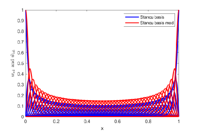
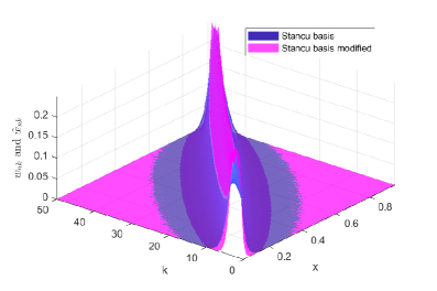
In Figure 1, we present the Stancu basis $w_{n,k}(x)$ and the Stancu basis modified $\widetilde{w}_{n,k}(x)=w_{n,k}^{2}(x)/(\sum_{k=0}^{n}w_{n,k}^{2}(x))$ for $n=50$ , while in Figure 2, we represent the same basis but in 3D and only for $x\in[0.05,\ 0.95]$ . We note that due to the form of the modified basis, the modified Stancu operators at point x give higher weights to values $f(k/n)$ closer to x and lower weights to values farther apart compared to the classical operators. This behavior is evident in the sharper peaks of the modified basis functions, which are more localized around their respective $k/n$ positions. We mention that this feature also applies to the other modified operators compared to the binomial classical ones, because the weights $\nu_{n,k}$ defined by the relation (22) have a form similar to $\widetilde{w}_{n,k}$ compared to the corresponding weights $p_{n,k}$ . This can be an advantage for certain functions and a disadvantage for others. For example, for functions that have a slower variation near the ends of the interval and faster in the rest, the residuals of the modified binomial operators are smaller than those of the classical binomial operators, which is illustrated in the following figures.

Refer to caption — Figure 1: The Stancu basis and Stancu basis modified for $n=50$ and $\alpha=1/n^{3/2}$ .

6.1 Example 1

This example refers to the approximation of the function

f_{1}(x)=sin(6x)log(x^{4}+1)tan((x-1)^{2}),\vskip-6.0pt

(26)

using binomial operators and modified binomial operators. First, in Figure 3, we present the shape of this function, the Stancu operators and modified Stancu operators with squared binomial polynomials for $n=20$ , $n=50$ , and $n=150$ for this function. We observe that the modified Stancu operators with squared binomial polynomials (plotted with dashed line) have a better approximation than the classical Stancu operators (plotted with continuous line) for the same $n$ , in this case, being closer to the function for almost all values of $x$ .

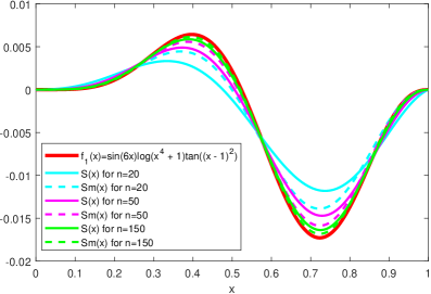
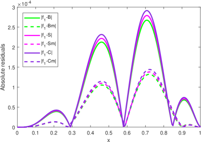
Figure 4 shows the absolute residual values for the operators: classical Bernstein ( $B$ ), modified Bernstein ( $B m$ ), classical Stancu ( $S$ ), modified Stancu ( $S m$ ), classical Cheney–Sharma ( $C$ ), and modified Cheney–Sharma ( $C m$ ) applied to the function $f_{1}$ defined by (26). First, we can see that the global maximum error for all operators occurs at the minimum point of the function $f_{1}$ , that is, at $x\approx 0.723$ , and the second maximum of the absolute residuals occurs at the maximum point of the function $x\approx 0.397$ . The minima for the classical binomial operators occur at the inflection points of the function, i.e., at $x\approx 0.2909$ , $x\approx 0.5799$ , and $x\approx 0.8476$ , while for the modified operators, the first minimum of the error is before the first inflection point and the last one is after the last inflection point. This is due to the fact that the operators are convex linear combinations of the values of the function $f(k/n)$ so that in the convexity areas of the function, the values of the operators are higher than the values of the function and in the concavity areas, the values of the operators are lower than the values of the function, and then the residual changes the sign around the inflection points of $f_{1}$ . We observe that the absolute residuals of the modified binomial operators are significantly smaller than those of their classical counterparts for almost all values of $x\in(0,1)$ (except for a few values around the inflection points of the function), so this function is better approximated by these operators. The same conclusion can be drawn from Table 1, where we have analyzed the absolute values of the residuals for the classical operators and for the modified ones for x from 0 to 1 with step 0.1. We mention that the values for the residuals for $x=0$ and for $x=1$ are 0 because all these operators interpolate the ends of the interval $[0,1]$ . In the interior of this interval for most values of $x$ , the absolute residual values of the modified operators are significantly lower than the absolute residuals of the classical operators. For example, at $x=0.1$ , the residual for $B m$ is approximately $36\%$ of the residual for $B$ . Also, at this point, the residual for $S m$ is approximately $36\%$ of the residual for $S$ . At $x=0.5$ , the residual for $B m$ is approximately $50\%$ of the residual for $B$ , and the residual for $S m$ is approximately $51\%$ of the residual for $S$ . At $x=0.9$ , the residual for $B m$ is approximately $4\%$ of the residual for $B$ , and the residual for $S m$ is approximately $18\%$ of the residual for $S$ . These ratios demonstrate that modified operators generally provide better approximation performance for this function, especially near the endpoints of the interval.

Table 1: Values of the absolute residuals for the classical and modified binomial operators for the function

f_{1}

defined by (26).

x	$\|f_{1}-B\|$	$\|f_{1}-Bm\|$	$\|f_{1}-S\|$	$\|f_{1}-Sm\|$	$\|f_{1}-C\|$	$\|f_{1}-Cm\|$
0.0	0	$0$	$0$	$0$	$0$	$0$
0.1	$8.316\times 10^{-6}$	$3.025\times 10^{-6}$	$8.698\times 10^{-6}$	$3.111\times 10^{-6}$	$9.098\times 10^{-6}$	$3.199\times 10^{-6}$
0.2	$3.829\times 10^{-5}$	$1.301\times 10^{-5}$	$3.997\times 10^{-5}$	$1.331\times 10^{-5}$	$4.172\times 10^{-5}$	$1.360\times 10^{-5}$
0.3	$1.189\times 10^{-5}$	$1.265\times 10^{-5}$	$1.249\times 10^{-5}$	$1.355\times 10^{-5}$	$1.313\times 10^{-5}$	$1.449\times 10^{-5}$
0.4	$1.659\times 10^{-4}$	$8.318\times 10^{-5}$	$1.733\times 10^{-4}$	$8.687\times 10^{-5}$	$1.809\times 10^{-4}$	$9.072\times 10^{-5}$
0.5	$1.871\times 10^{-4}$	$9.459\times 10^{-5}$	$1.952\times 10^{-4}$	$9.878\times 10^{-5}$	$2.038\times 10^{-4}$	$1.031\times 10^{-4}$
0.6	$6.302\times 10^{-5}$	$2.014\times 10^{-5}$	$6.580\times 10^{-5}$	$2.053\times 10^{-5}$	$6.870\times 10^{-5}$	$2.091\times 10^{-5}$
0.7	$2.662\times 10^{-4}$	$1.282\times 10^{-4}$	$2.779\times 10^{-4}$	$1.336\times 10^{-4}$	$2.901\times 10^{-4}$	$1.393\times 10^{-4}$
0.8	$1.188\times 10^{-4}$	$8.526\times 10^{-5}$	$1.241\times 10^{-4}$	$9.020\times 10^{-5}$	$1.297\times 10^{-4}$	$9.541\times 10^{-5}$
0.9	$6.630\times 10^{-5}$	$2.352\times 10^{-7}$	$6.917\times 10^{-5}$	$1.258\times 10^{-6}$	$7.217\times 10^{-5}$	$2.885\times 10^{-6}$
1.0	$0$	$0$	$0$	$0$	$0$	$0$

We mention that the run time on an HP computer having an Intel(R) Core(TM) i5-6500 CPU @ 3.20 GHz processor for computing the values of the operators $S$ and $S m$ applied to $f_{1}$ on 500 values of $x$ was: 1.77 s for $n=100$ , 5.29 s for $n=300$ , and t = 8.48 s for $n=500$ . Similar run times were obtained for the other operators studied in this paper.

6.2 Example 2

In our second example, we analyze the approximation of the function

f_{2}(x)=(sin(x)sin(1-x))^{3},\vskip-6.0pt

(27)

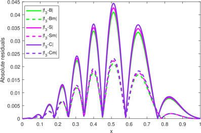
using binomial operators and modified binomial operators. Figure 5 shows the absolute residual values for this function for the binomial operators Bernstein, Stancu, and Cheney–Sharma and for their modified versions involving squared binomial polynomials ( $B m$ , $S m$ , and $C m$ ). Similarly to the behavior discussed for Figure 4, we can see that the global maximum error for all operators occurs at the maximum point of the function $f_{2}(x)$ , that is, at x = 0.5. The minima of the error for the classical binomial operators occur at the inflection points of the function, i.e., at $x\approx 0.2881$ and $x\approx 0.7119$ , while for the modified operators, the first minima of the error is before the first inflection point and the second one is after the second inflection point. We observe that the absolute residuals of the modified binomial operators are much smaller than those of the classical operators for almost all values of $x\in(0,1)$ (except for a small interval around 0.3 and 0.7, i.e., in the neighborhood of the inflection points of the function), so this function is better approximated by these operators. The same conclusion can be drawn from Table 2, where we have analyzed the absolute values of the residuals for the classical binomial operators and for the modified ones for x from 0 to 1 with step 0.1 (see also the first four columns of Table 4). We can remark that for the values of x in $(0,0.21)$ and $(0.73,1)$ , the errors for modified operators are less than a quarter of the errors for classical binomial operators analyzed, indicating better performance of the modified operators near the endpoints. More specifically, at $x=0.2$ , the residuals for the modified operators range from approximately 9% to 12.5% of the residuals for the classical operators, at $x=0.8$ , the residuals for the modified operators are less than 13% of the residuals for the classical operators and at $x=0.9$ , the residuals for the modified operators are less than 23% of the residuals for the classical operators. Around $x=0.3$ and $x=0.7$ , the ratios of the absolute residuals are around 2, indicating that the modified operators perform worse than the classical ones in the region around the inflection points of the function. At x = 0.5, the ratios are approximately 0.5, which shows that the modified operators reduce the residuals by about 50% at the global maximum of the function. So, the modified operators ( $B m$ , $S m$ , $C m$ ) generally exhibit smaller residuals compared to their classical counterparts ( $B$ , $S$ , $C$ ) for most values of x for this function.

Table 2: Values of the absolute residuals for the classical and modified operators for the function

f_{2}

defined by (27).

x	$\|f_{2}-B\|$	$\|f_{2}-Bm\|$	$\|f_{2}-S\|$	$\|f_{2}-Sm\|$	$\|f_{2}-C\|$	$\|f_{2}-Cm\|$
0.0	$0$	$0$	$0$	$0$	$0$	$0$
0.1	$1.936\times 10^{-5}$	$4.431\times 10^{-6}$	$2.022\times 10^{-5}$	$4.391\times 10^{-6}$	$2.112\times 10^{-5}$	$4.339\times 10^{-6}$
0.2	$2.723\times 10^{-5}$	$3.408\times 10^{-6}$	$2.843\times 10^{-5}$	$3.096\times 10^{-6}$	$2.968\times 10^{-5}$	$2.750\times 10^{-6}$
0.3	$5.821\times 10^{-6}$	$1.131\times 10^{-5}$	$6.093\times 10^{-6}$	$1.220\times 10^{-5}$	$6.378\times 10^{-6}$	$1.314\times 10^{-5}$
0.4	$5.542\times 10^{-5}$	$3.068\times 10^{-5}$	$5.788\times 10^{-5}$	$3.218\times 10^{-5}$	$6.045\times 10^{-5}$	$3.375\times 10^{-5}$
0.5	$7.869\times 10^{-5}$	$3.952\times 10^{-5}$	$8.218\times 10^{-5}$	$4.128\times 10^{-5}$	$8.582\times 10^{-5}$	$4.312\times 10^{-5}$
0.6	$5.542\times 10^{-5}$	$3.068\times 10^{-5}$	$5.788\times 10^{-5}$	$3.218\times 10^{-5}$	$6.045\times 10^{-5}$	$3.375\times 10^{-5}$
0.7	$5.821\times 10^{-6}$	$1.131\times 10^{-5}$	$6.093\times 10^{-6}$	$1.220\times 10^{-5}$	$6.378\times 10^{-6}$	$1.314\times 10^{-5}$
0.8	$2.723\times 10^{-5}$	$3.408\times 10^{-6}$	$2.843\times 10^{-5}$	$3.096\times 10^{-6}$	$2.968\times 10^{-5}$	$2.750\times 10^{-6}$
0.9	$1.936\times 10^{-5}$	$4.431\times 10^{-6}$	$2.022\times 10^{-5}$	$4.391\times 10^{-6}$	$2.112\times 10^{-5}$	$4.339\times 10^{-6}$
1.0	$0$	$0$	$0$	$0$	$0$	$0$

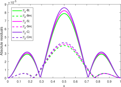
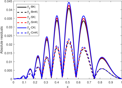
Figure 6 and Table 3 compare the absolute residuals for the classical binomial Kantorovich operators and for those involving squared binomial polynomials. We remark that at endpoints, we have very small but non-zero residuals ( $1.181\times 10^{-9}$ ) for all operators, since Kantorovich-type operators do not interpolate endpoints exactly. For all interior points, the modified Kantorovich operators with quadratic binomial polynomials consistently produce residuals about half the size of classical versions, so the conclusion we can draw is that the latter approximate this function better than the others.

Table 3: Values of the absolute residuals for the classical and modified operators of Kantorovich type for the function

f_{2}

defined by (27).

x	$\|f_{2}-BK\|$	$\|f_{2}-BmK\|$	$\|f_{2}-SK\|$	$\|f_{2}-SmK\|$	$\|f_{2}-CK\|$	$\|f_{2}-CmK\|$
0.0	$1.181\times 10^{-9}$	$1.181\times 10^{-9}$	$1.181\times 10^{-9}$	$1.181\times 10^{-9}$	$1.181\times 10^{-9}$	$1.181\times 10^{-9}$
0.1	$2.995\times 10^{-5}$	$1.497\times 10^{-5}$	$3.081\times 10^{-5}$	$1.493\times 10^{-5}$	$3.171\times 10^{-5}$	$1.487\times 10^{-5}$
0.2	$4.765\times 10^{-5}$	$2.394\times 10^{-5}$	$4.883\times 10^{-5}$	$2.362\times 10^{-5}$	$5.007\times 10^{-5}$	$2.326\times 10^{-5}$
0.3	$1.091\times 10^{-5}$	$5.521\times 10^{-6}$	$1.063\times 10^{-5}$	$4.635\times 10^{-6}$	$1.034\times 10^{-5}$	$3.693\times 10^{-6}$
0.4	$4.957\times 10^{-5}$	$2.489\times 10^{-5}$	$5.203\times 10^{-5}$	$2.638\times 10^{-5}$	$5.459\times 10^{-5}$	$2.795\times 10^{-5}$
0.5	$7.843\times 10^{-5}$	$3.942\times 10^{-5}$	$8.191\times 10^{-5}$	$4.117\times 10^{-5}$	$8.553\times 10^{-5}$	$4.300\times 10^{-5}$
0.6	$4.957\times 10^{-5}$	$2.489\times 10^{-5}$	$5.203\times 10^{-5}$	$2.638\times 10^{-5}$	$5.459\times 10^{-5}$	$2.795\times 10^{-5}$
0.7	$1.091\times 10^{-5}$	$5.521\times 10^{-6}$	$1.063\times 10^{-5}$	$4.635\times 10^{-6}$	$1.034\times 10^{-5}$	$3.693\times 10^{-6}$
0.8	$4.765\times 10^{-5}$	$2.394\times 10^{-5}$	$4.883\times 10^{-5}$	$2.362\times 10^{-5}$	$5.007\times 10^{-5}$	$2.326\times 10^{-5}$
0.9	$2.995\times 10^{-5}$	$1.497\times 10^{-5}$	$3.081\times 10^{-5}$	$1.493\times 10^{-5}$	$3.171\times 10^{-5}$	$1.487\times 10^{-5}$
1.0	$1.181\times 10^{-9}$	$1.181\times 10^{-9}$	$1.181\times 10^{-9}$	$1.181\times 10^{-9}$	$1.181\times 10^{-9}$	$1.181\times 10^{-9}$

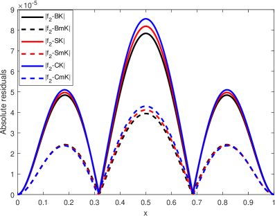
Table 4 presents the ratios between the absolute residuals for modified operators and their classical counterparts applied to the function $f_{2}(x)=(sin(x)sin(1-x))^{3}$ for different values of $x$ (from 0.1 to 0.9, with a step of 0.1). The columns from 2 to 4 display ratios for three types of modified operators versus classical ones,

r_{2}(Bm,B)=\frac{|f_{2}-Bm|}{|f_{2}-B|},\ \ r_{2}(Sm,S)=\frac{|f_{2}-Sm|}{|f_% {2}-S|},\ \ r_{2}(Cm,C)=\frac{|f_{2}-Cm|}{|f_{2}-C|},\vskip-6.0pt

while columns from 5 to 7 show similar ratios, but for the modified Kantorovich type versus the classical Kantorovich ones, i.e.,

r_{2}(BmK,BK)=\frac{|f_{2}-BmK|}{|f_{2}-BK|},\ \ r_{2}(SmK,S)=\frac{|f_{2}-SmK% |}{|f_{2}-SK|}\ \ \text{and}\ \ r_{2}(CmK,CK)=\frac{|f_{2}-CmK|}{|f_{2}-CK|}.% \vskip-6.0pt

Blue values are values smaller than one, indicating smaller residuals for the modified operators, suggesting better approximations, while red values indicate larger residuals for modified operators, suggesting less accurate approximations.

Table 4: Ratios between the absolute residuals for modified operators and their classical counterparts for the function

f_{2}

defined by (27).

x	$r_{2}(Bm,B)$	$r_{2}(Sm,S)$	$r_{2}(Cm,C)$	$r_{2}(BmK,BK)$	$r_{2}(SmK,SK)$	$r_{2}(CmK,CK)$
0.1	0.2289	0.2172	0.2054	0.4998	0.4846	0.4698
0.2	0.1252	0.1089	0.0927	0.5024	0.4837	0.4645
0.3	1.9430	2.0023	2.0602	0.5060	0.4360	0.3572
0.4	0.5536	0.5560	0.5583	0.5021	0.5070	0.5120
0.5	0.5022	0.5023	0.5024	0.5026	0.5026	0.5027
0.6	0.5536	0.5560	0.5583	0.5021	0.5070	0.5120
0.7	1.9430	2.0023	2.0602	0.5060	0.4360	0.3572
0.8	0.1252	0.1089	0.0927	0.5024	0.4837	0.4645
0.9	0.2289	0.2172	0.2054	0.4998	0.4846	0.4689

6.3 Example 3

In this example, we consider the following function

f_{3}(x)=x^{2}exp(x^{3}-x^{5})cos(8\pi x),\vskip-6.0pt

(28)

that exhibits several local extrema, allowing us to further illustrate the strengths and limitations of the operators discussed. The comparison will focus on the accuracy of the classical and modified operators, as well as their Kantorovich variants, in approximating this function across the interval $[0,\,1]$ .

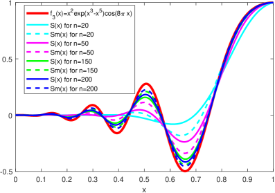
Figure 7 presents the shape of the function $f_{3}$ , along with the Stancu operators and modified Stancu operators with squared binomial polynomials for $n\in\{20,50,150,200\}$ . The function $f_{3}$ has three maxima and three minima in the interior of the interval $[0,\,1]$ . Analogously to the other functions, analyzing the absolute residuals of the function $f_{3}$ in Figure 8, we can see that the maxima of the error for all operators occur at the extrema points of the function $f_{3}$ . Modified Stancu operators (dashed lines) show a closer approximation to the function than the classical Stancu operators (solid lines) for the same $n$ . Moreover, for example, the modified operator for $n=150$ performs better than the classical operator for $n=200$ . Similar conclusions can be drawn for the other modified operators compared to the classical ones.

Table 5: Values of the absolute residuals for the classical and modified operators for the function

f_{3}

defined by (28) for

n=500

x	$\|f_{3}-B\|$	$\|f_{3}-Bm\|$	$\|f_{3}-S\|$	$\|f_{3}-Sm\|$	$\|f_{3}-C\|$	$\|f_{3}-Cm\|$
0.0	$0$	$0$	$0$	$0$	$0$	$0$
0.1	$1.199\times 10^{-3}$	$4.954\times 10^{-4}$	$1.239\times 10^{-3}$	$5.068\times 10^{-4}$	$1.280\times 10^{-3}$	$5.181\times 10^{-4}$
0.2	$7.017\times 10^{-3}$	$3.888\times 10^{-3}$	$7.311\times 10^{-3}$	$4.066\times 10^{-3}$	$7.615\times 10^{-3}$	$4.250\times 10^{-3}$
0.3	$2.183\times 10^{-2}$	$1.159\times 10^{-2}$	$2.268\times 10^{-2}$	$1.207\times 10^{-2}$	$2.356\times 10^{-2}$	$1.257\times 10^{-2}$
0.4	$3.373\times 10^{-2}$	$1.773\times 10^{-2}$	$3.506\times 10^{-2}$	$1.847\times 10^{-2}$	$3.644\times 10^{-2}$	$1.924\times 10^{-2}$
0.5	$3.921\times 10^{-2}$	$2.042\times 10^{-2}$	$4.081\times 10^{-2}$	$2.130\times 10^{-2}$	$4.248\times 10^{-2}$	$2.221\times 10^{-2}$
0.6	$1.599\times 10^{-2}$	$7.622\times 10^{-3}$	$1.664\times 10^{-2}$	$7.917\times 10^{-3}$	$1.732\times 10^{-2}$	$8.221\times 10^{-3}$
0.7	$2.143\times 10^{-2}$	$1.188\times 10^{-2}$	$2.238\times 10^{-2}$	$1.246\times 10^{-2}$	$2.336\times 10^{-2}$	$1.306\times 10^{-2}$
0.8	$6.836\times 10^{-3}$	$1.256\times 10^{-3}$	$7.126\times 10^{-3}$	$1.208\times 10^{-3}$	$7.427\times 10^{-3}$	$1.154\times 10^{-3}$
0.9	$3.616\times 10^{-3}$	$8.399\times 10^{-4}$	$3.779\times 10^{-3}$	$8.341\times 10^{-4}$	$3.950\times 10^{-3}$	$8.260\times 10^{-4}$
1.0	$0$	$0$	$0$	$0$	$0$	$0$

Figure 8 displays the absolute residuals for the classical and modified operators (Bernstein, Stancu, Cheney–Sharma, and their modified versions) when approximating the function $f_{3}$ for $n=500$ . The plot shows that, for almost all values of $x\in(0,1)$ , the modified operators (those involving squared binomial polynomials) yield significantly smaller absolute residuals compared to their classical counterparts. The largest errors for all operators are observed at the extrema of the function, while the residuals are minimized near the endpoints and at certain interior points. This figure and Table 5 show that the modified operators provide a more accurate approximation of $f_{3}$ across most of the interval, especially near the endpoints, with the exception of small neighborhoods around inflection points (visible in the figure before $x=0.8$ , i.e, in the vicinity of the last inflection point of this function in [0, 1]), where the classical operators perform similarly or slightly better. A similar behavior can be seen in Figure 9, which displays the absolute residuals for the classical binomial Kantorovich operators (BK, SK, CK) and their modified counterparts involving squared binomial polynomials (BmK, SmK, CmK) when approximating the function $f_{3}$ , defined by Equation (28) for $n=500$ (see also Table 6 and the last three columns of Table 7).

Table 6: Values of the absolute residuals for the classical and modified operators of Kantorovich type for

n=500

for the function

f_{3}

x	$\|f_{3}-BK\|$	$\|f_{3}-BmK\|$	$\|f_{3}-SK\|$	$\|f_{3}-SmK\|$	$\|f_{3}-CK\|$	$\|f_{3}-CmK\|$
0.0	$1.324\times 10^{-6}$	$1.324\times 10^{-6}$	$1.324\times 10^{-6}$	$1.324\times 10^{-6}$	$1.324\times 10^{-6}$	$1.324\times 10^{-6}$
0.1	$1.518\times 10^{-3}$	$8.395\times 10^{-4}$	$1.556\times 10^{-3}$	$8.492\times 10^{-4}$	$1.594\times 10^{-3}$	$8.587\times 10^{-4}$
0.2	$6.623\times 10^{-3}$	$3.407\times 10^{-3}$	$6.922\times 10^{-3}$	$3.587\times 10^{-3}$	$7.233\times 10^{-3}$	$3.775\times 10^{-3}$
0.3	$2.191\times 10^{-2}$	$1.167\times 10^{-2}$	$2.276\times 10^{-2}$	$1.215\times 10^{-2}$	$2.363\times 10^{-2}$	$1.265\times 10^{-2}$
0.4	$3.383\times 10^{-2}$	$1.789\times 10^{-2}$	$3.517\times 10^{-2}$	$1.863\times 10^{-2}$	$3.654\times 10^{-2}$	$1.940\times 10^{-2}$
0.5	$3.909\times 10^{-2}$	$2.037\times 10^{-2}$	$4.069\times 10^{-2}$	$2.124\times 10^{-2}$	$4.234\times 10^{-2}$	$2.215\times 10^{-2}$
0.6	$1.728\times 10^{-2}$	$9.008\times 10^{-3}$	$1.792\times 10^{-2}$	$9.298\times 10^{-3}$	$1.859\times 10^{-2}$	$9.598\times 10^{-3}$
0.7	$1.926\times 10^{-2}$	$9.683\times 10^{-3}$	$2.021\times 10^{-2}$	$1.026\times 10^{-2}$	$2.120\times 10^{-2}$	$1.086\times 10^{-2}$
0.8	$1.126\times 10^{-2}$	$5.719\times 10^{-3}$	$1.154\times 10^{-2}$	$5.669\times 10^{-3}$	$1.184\times 10^{-2}$	$5.613\times 10^{-3}$
0.9	$5.565\times 10^{-3}$	$2.771\times 10^{-3}$	$5.729\times 10^{-3}$	$2.765\times 10^{-3}$	$5.900\times 10^{-3}$	$2.756\times 10^{-3}$
1.0	$1.061\times 10^{-5}$	$1.061\times 10^{-5}$	$1.061\times 10^{-5}$	$1.061\times 10^{-5}$	$1.061\times 10^{-5}$	$1.061\times 10^{-5}$

Table 7, similar to Table 4, presents the ratios of absolute residuals for modified operators to their classical counterparts, evaluated for the function $f_{3}$ (denoted by $r_{3}(Bm,B)$ etc.) at points $x$ from 0.1 to 0.9 in steps of 0.1. All ratios for these points are less than 1 (displayed in blue), indicating that the modified operators consistently produce smaller absolute residuals than their classical counterparts for all $x$ values shown. The ratios are generally between 0.15 and 0.56, showing a significant reduction in residuals. The lowest ratios occur at $x=0.8$ and $x=0.9$ for $B m$ versus $B$ , $S m$ versus $S$ , and $C m$ versus $C$ , showing that modified operators are especially effective at these points. The Kantorovich-type ratios are also below 1, in fact, they are below 0.56, but tend to be slightly higher than the corresponding non-Kantorovich ratios, indicating a smaller (but still present) improvement. The modified operators outperform their classical counterparts in terms of absolute residuals across the interval [0, 1] for the function $f_{3}$ defined by the relation (28), the improvement being more pronounced at higher $x$ values.

Table 7: Ratios between the absolute residuals for modified operators and their classical counterparts for

n=500

for the function

f_{3}

x	$r_{3}(Bm,B)$	$r_{3}(Sm,S)$	$r_{3}(Cm,C)$	$r_{3}(BmK,BK)$	$r_{3}(SmK,SK)$	$r_{3}(CmK,CK)$
0.1	0.4131	0.4089	0.4048	0.5529	0.5458	0.5388
0.2	0.5541	0.5561	0.5581	0.5144	0.5182	0.5219
0.3	0.5308	0.5321	0.5335	0.5326	0.5339	0.5351
0.4	0.5256	0.5268	0.5280	0.5287	0.5297	0.5308
0.5	0.5210	0.5219	0.5229	0.5212	0.5221	0.5231
0.6	0.4767	0.4757	0.4748	0.5213	0.5188	0.5163
0.7	0.5546	0.5569	0.5591	0.5027	0.5076	0.5124
0.8	0.1837	0.1696	0.1554	0.5080	0.4911	0.4741
0.9	0.2323	0.2207	0.2091	0.4979	0.4826	0.4671

6.4 Example 4

In this example, we shall present the approximation of the following function with two jump discontinuities

f_{4}(x)=\begin{cases}\frac{4x^{2}}{x+1},&\text{for }x\in[0,1/2],\\ \sqrt{x},&\text{for }x\in(1/2,3/4],\\ \sin(3x/2),&\text{for }x\in(3/4,1],\end{cases}\vskip-6.0pt

(29)

using the classical Kantorovich and modified Kantorovich operators defined by (9) and (21), respectively.

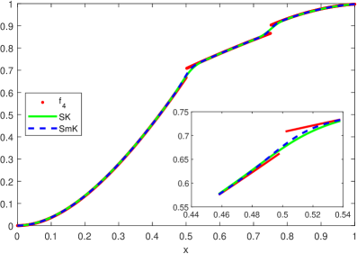
In Figure 10, we represented this function and Stancu–Kantorovich operators and modified Stancu–Kantorovich operators with squared binomial polynomials for $n=500$ applied to this function, while in Figure 11, we plotted the absolute residual values for six operators for $n=500$ .

For better visibility, in the smaller figure inserted in Figure 10, we zoomed in on the zone around the first discontinuity point $x=0.5$ .

As expected, the maxima of the error occurs at the discontinuity points, and their values are a fraction of the height of the jumps because the operators and their modified versions have a smooth transition from the values located on the left of the discontinuity points to the values situated to the right.

One can observe that for most values of $x\in(0,\ 1)$ , the residuals for modified Kantorovich operators (plotted with dashed line) are smaller than the residuals for their classical counterparts (plotted with continuous line).

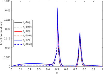
In Table 8, we show the values of the absolute residuals for three classical binomial-type Kantorovich operators and for their modified versions. Besides the values from 0 to 0.9 with step 0.1 displayed in the previous tables, we added the value x = 0.502 situated to the right of the first discontinuity point to emphasize that if the values of the operators $B K$ , $S K$ , and $C K$ at the left of the jump discontinuity point x = 0.5 are closer to the function than the values of $B m K$ , $S m K$ , and $C m K$ , in the right proximity of this point are closer to the function than their classical corresponding ones (because of their smooth transition mentioned above).

Table 8: Values of the absolute residuals for the classical and modified operators of Kantorovich type for

n=500

for the function

f_{4}

x	$\|f_{4}-BK\|$	$\|f_{4}-BmK\|$	$\|f_{4}-SK\|$	$\|f_{4}-SmK\|$	$\|f_{4}-CK\|$	$\|f_{4}-CmK\|$
0.0	$5.304\times 10^{-6}$	$5.304\times 10^{-6}$	$5.304\times 10^{-6}$	$5.304\times 10^{-6}$	$5.304\times 10^{-6}$	$5.304\times 10^{-6}$
0.1	$1.094\times 10^{-3}$	$5.471\times 10^{-4}$	$1.118\times 10^{-3}$	$5.341\times 10^{-4}$	$1.143\times 10^{-3}$	$5.200\times 10^{-4}$
0.2	$1.470\times 10^{-3}$	$7.353\times 10^{-4}$	$1.503\times 10^{-3}$	$7.189\times 10^{-4}$	$1.537\times 10^{-3}$	$7.011\times 10^{-4}$
0.3	$1.414\times 10^{-3}$	$7.073\times 10^{-4}$	$1.448\times 10^{-3}$	$6.951\times 10^{-4}$	$1.483\times 10^{-3}$	$6.818\times 10^{-4}$
0.4	$1.089\times 10^{-3}$	$5.446\times 10^{-4}$	$1.120\times 10^{-3}$	$5.427\times 10^{-4}$	$1.152\times 10^{-3}$	$5.403\times 10^{-4}$
0.5	$6.942\times 10^{-3}$	$1.078\times 10^{-2}$	$6.654\times 10^{-3}$	$1.057\times 10^{-2}$	$6.360\times 10^{-3}$	$1.036\times 10^{-2}$
0.502	$3.065\times 10^{-2}$	$2.623\times 10^{-2}$	$3.097\times 10^{-2}$	$2.648\times 10^{-2}$	$3.130\times 10^{-2}$	$2.673\times 10^{-2}$
0.6	$2.579\times 10^{-4}$	$1.289\times 10^{-4}$	$2.638\times 10^{-4}$	$1.260\times 10^{-4}$	$2.699\times 10^{-4}$	$1.228\times 10^{-4}$
0.7	$9.984\times 10^{-5}$	$1.561\times 10^{-4}$	$6.747\times 10^{-5}$	$1.449\times 10^{-4}$	$3.116\times 10^{-5}$	$1.324\times 10^{-4}$
0.8	$7.849\times 10^{-4}$	$3.324\times 10^{-4}$	$8.243\times 10^{-4}$	$3.262\times 10^{-4}$	$8.679\times 10^{-4}$	$3.197\times 10^{-4}$
0.9	$4.600\times 10^{-4}$	$2.298\times 10^{-4}$	$4.688\times 10^{-4}$	$2.224\times 10^{-4}$	$4.780\times 10^{-4}$	$2.144\times 10^{-4}$
1.0	$1.074\times 10^{-4}$	$1.074\times 10^{-4}$	$1.074\times 10^{-4}$	$1.074\times 10^{-4}$	$1.074\times 10^{-4}$	$1.074\times 10^{-4}$

7 Discussion

The conclusion is that the modified binomial operators are more efficient than the classical ones for approximating functions with specific characteristics, particularly those that exhibit slower variation near the ends of the interval and have fluctuations in the rest. This is because the modified operators at a point $x$ situated within the interval [0, 1] (and not very close to the endpoints) give higher weights to values $f(k/n)$ closer to $x$ and lower weights to values farther apart compared to the classical operators. For other functions, the results may vary, and further analysis is needed to determine the best operator choice for specific applications. For some values of $x$ close to the ends of the interval, the values of the modified weights are more asymmetrical in the sense that for the left end, the values of the weights that multiply the values $f(k/n)$ for $k/n$ located at the left of the point x are much larger than the values of the weights that multiply the values $f(k/n)$ for $k/n$ located at the right of the point x, so the computed values of the modified operators take into account the greater weight values of the function to the left of the current value than those to the right. So, for functions that vary rapidly at the endpoints, this behavior will lead to a deviation of the value of the operator at that point from the value of the function, i.e., to higher residuals. Therefore, for functions with rapid variation near the endpoints, classical operators may yield better results in these areas. Similar observations hold for Kantorovich-type operators. The choice between classical and modified operators should, therefore, be guided by the specific properties of the target function.

As a future direction, we mention that we can define and study similar modified operators for the classes of operators constructed using binomial and Sheffer sequences considered in [11, 12].

Finally, it is important to mention a new active research field in the use of polynomial-type operators to obtain solutions to differential equations. In Ref. [25], the authors combine polynomial approximation to derive a piecewise polynomial representation similar to a spline function. This technique improves the inference on system properties. Using a polynomial LD basis (see Remark 4(i)) in [26], nonlinear partial differential equations that arise in various fields have been solved. In support of our claims, one can also consult [27].

8 Conclusions

The paper is focused on binomial polynomials, and their applications in the construction of linear and positive approximation operators.

Starting from the classical operators, three new classes of discrete or continuous operators are investigated. The results obtained aim at the evaluation of the absolute error in $L_{p}([0,1]),\ p\geq 1$ , spaces generated by a Kantorovich integral extension, the introduction of a discrete class involving squared binomial basis polynomials accompanied by the study of uniform convergence in $C([0,1])$ , as well as its generalization in the integral sense with the evaluation of the maximum error, again in $L_{p}([0,1])$ spaces.

The numerical results presented contain the approximation of some specific functions using operators belonging to the classes of operators studied. The results obtained are analyzed in detail, highlighting the usefulness of the new sequences and pointing out their pros and cons.

Acknowledgements

During the preparation of this manuscript/study, the second author used the latexTable function of Eli Duenisch (https://github.com/eliduenisch/latexTable) and the copilot from Visual Studio Code, version: 1.102.1. for the purpose of rephrasing the text and describing the tables. The authors have reviewed and edited the output and take full responsibility for the content of this publication.

References

[1] Mullin, I.R.; Rota, G.-C. On the Foundations of Combinatorial Theory. III. Theory of binomial enumeration. In Graph Theory and Its Applications; Harris, B., Ed.; Academic Press: Cambridge, MA, USA, 1970; pp. 167–213.
[2] Rota, G.-C.; Kahaner, D.; Odlyzko, A. On the Foundations of Combinatorial Theory. VIII. Finite operator calculus. J. Math. Anal. Appl. 1973, 42, 685–760.
[3] Sablonniere, P. Positive Bernstein-Sheffer operators. J. Approx. Theory 1995, 83, 330–341.
[4] Stancu, D.D.; Occorsio, M.R. On approximation by binomial operators of Tiberiu Popoviciu type Rev. Roum. Math. Pures Appl. 1998, 27, 167–181.
[5] Popoviciu, T. Remarques sur les polynômes binomiaux. Bull. Soc. Sci. Cluj 1931, 6, 146–148; reprinted in Mathematica 1932, 6, 8–10.
[6] Stancu, D.D. Approximation of functions by a new class of linear operators. Rev. Roum. Math. Pures Appl. 1968, 13, 1173–1194.
[7] Cheney, E.W.; Sharma, A. On a generalization of Bernstein polynomials. Riv. Math. Univ. Parma 1964, 5, 77–84.
[8] Lupaş, L.; Lupaş, A. Polynomials of binomial type and approximation operators. Stud. Univ. Babeş-Bolyai Math. 1987, 32, 61–69.
[9] Agratini, O.; Rus, I.A. Iterates of a class of discrete operators via contraction principle. Comment. Math. Univ. Carolin. 2003, 44, 555–563.
[10] Agratini, O. On a certain class of approximation operators. Pure Math. Appl. 2000, 11, 119–127.
[11] Crăciun, M. Approximation operators constructed by means of Sheffer sequences. Rev. Anal. Numér. Théor. Approx. 2001, 30, 135–150.
[12] Crăciun, M. Note on an approximation operator and its Lipschitz constant, Rev. Anal. Numér. Théor. Approx. 2002, 31, 55–60.
[13] Altomare, F.; Campiti, M. Korovkin-Type Approximation Theory and Its Applications; de Gruyter Series Studies in Mathematics; Walter de Gruyter: Berlin, Germany; New York, NY, USA, 1994; Volume 17.
[14] Peetre, J. A Theory of Interpolation of Normed Spaces; Notes Universidade de Brasilia: Brasília, Brazil, 1963.
[15] Johnen, H. Inequalities connected with the moduli of smoothness. Math. Vesnik 1972, 24, 289–305.
[16] Stein, E.M. Singular Integrals and Differentiability Properties of Functions; Princeton University Press: Princeton, NJ, USA, 1970.
[17] Swetits, J.J.; Wood, B. Note on the degree of $L_{p}$ approximation with positive linear operators. J. Approx. Theory 1996, 87, 239–241.
[18] Abel, U. Voronovskaja Type Theorems for Positive Linear Operators Related to Squared Fundamental Functions. In Constructive Theory of Functions, Proceedings of the Constructive Theory of Functions, Sozopol, Bulgaria, 2–8 June 2019 ; Draganov, B., Ivanov, K., Nikolov, G., Uluchev, R., Eds.; Prof. Marin Drinov Publishing House of BAS: Sofia, Bulgaria, 2020; pp. 1–21.
[19] Herzog, F. Heuristische Untersuchungen der Konvergenzrate Spezieller Linearer Approximationsprozesse. Ph.D. Thesis, Friedberg University, Germany 2009.
[20] Gavrea, I.; Ivan, M. On a new sequence of positive linear operators related to squared Bernstein polynomials. Positivity 2017, 21, 911–917.
[21] Holhoş, A. Voronovskaya theorem for a sequence of positive linear operators related to squared Bernstein polynomials. Positivity 2019, 23, 571–580.
[22] Harremoes, P.; Topsoe, F. Inequalities between entropy and index of coincidence derrived from information diagrams. IEEE Trans. Inf. Theory 2001, 47, 2944–2960.
[23] Shisha, O.; Mond, B. The degree of convergence of linear positive operators. Proc. Natl. Acad. Sci. USA 1968, 60, 1196–1200.
[24] Shin, C.E.; Sun, Q. Stability of the localized operators. J. Funct. Anal. 2009, 256, 2417–2439.
[25] Martin, T.; Allgöwer, F. Data-Driven System Analysis of Nonlinear Systems Using Polynomial Approximation. IEEE Trans. Autom. Control 2024, 69, 4261–4274.
[26] Bhatti, M.I.; Rahman, M.H.; Dimakis, N. Approximate Solutions of Nonlinear Partial Differential Equations Using B-Polynomial Bases. Fractal Fract. 2021, 5, 106.
[27] El Yazidi, Y.; Ellabib, A. An Efficient Numerical Scheme Based on Radial Basis Functions and a Hybrid Quasi-Newton Method for a Nonlinear Shape Optimization Problem. Math. Comput. Appl. 2022, 27, 67.

Mullin, I.R.; Rota, G.-C. On the Foundations of Combinatorial Theory. III. Theory of binomial enumeration. In Graph Theory and Its Applications; Harris, B., Ed.; Academic Press: Cambridge, MA, USA, 1970; pp. 167–213. [Google Scholar]
Rota, G.-C.; Kahaner, D.; Odlyzko, A. On the Foundations of Combinatorial Theory. VIII. Finite operator calculus. J. Math. Anal. Appl. 1973, 42, 685–760. [Google Scholar] [CrossRef]
Sablonniere, P. Positive Bernstein-Sheffer operators. J. Approx. Theory 1995, 83, 330–341. [Google Scholar] [CrossRef]
Stancu, D.D.; Occorsio, M.R. On approximation by binomial operators of Tiberiu Popoviciu type. Rev. Roum. Math. Pures Appl. 1998, 27, 167–181. [Google Scholar]
Popoviciu, T. Remarques sur les polynômes binomiaux. Bull. Soc. Sci. Cluj 1931, 6, 146–148, reprinted in Mathematica 1932, 6, 8–10. [Google Scholar]
Stancu, D.D. Approximation of functions by a new class of linear operators. Rev. Roum. Math. Pures Appl. 1968, 13, 1173–1194. [Google Scholar]
Cheney, E.W.; Sharma, A. On a generalization of Bernstein polynomials. Riv. Math. Univ. Parma 1964, 5, 77–84. [Google Scholar]
Lupaş, L.; Lupaş, A. Polynomials of binomial type and approximation operators. Stud. Univ. Babeş-Bolyai Math. 1987, 32, 61–69. [Google Scholar]
Agratini, O.; Rus, I.A. Iterates of a class of discrete operators via contraction principle. Comment. Math. Univ. Carolin. 2003, 44, 555–563. [Google Scholar]
Agratini, O. On a certain class of approximation operators. Pure Math. Appl. 2000, 11, 119–127. [Google Scholar]
Crăciun, M. Approximation operators constructed by means of Sheffer sequences. Rev. Anal. Numér. Théor. Approx. 2001, 30, 135–150. [Google Scholar] [CrossRef]
Crăciun, M. Note on an approximation operator and its Lipschitz constant. Rev. Anal. Numér. Théor. Approx. 2002, 31, 55–60. [Google Scholar] [CrossRef]
Altomare, F.; Campiti, M. Korovkin-Type Approximation Theory and Its Applications; de Gruyter Series Studies in Mathematics; Walter de Gruyter: Berlin, Germany; New York, NY, USA, 1994; Volume 17. [Google Scholar]
Peetre, J. A Theory of Interpolation of Normed Spaces; Notes Universidade de Brasilia: Brasília, Brazil, 1963. [Google Scholar]
Johnen, H. Inequalities connected with the moduli of smoothness. Math. Vesnik 1972, 24, 289–305. [Google Scholar]
Stein, E.M. Singular Integrals and Differentiability Properties of Functions; Princeton University Press: Princeton, NJ, USA, 1970. [Google Scholar]
Swetits, J.J.; Wood, B. Note on the degree of L_p approximation with positive linear operators. J. Approx. Theory 1996, 87, 239–241. [Google Scholar] [CrossRef]
Abel, U. Voronovskaja Type Theorems for Positive Linear Operators Related to Squared Fundamental Functions. In Constructive Theory of Functions, Proceedings of the Constructive Theory of Functions, Sozopol, Bulgaria, 2–8 June 2019; Draganov, B., Ivanov, K., Nikolov, G., Uluchev, R., Eds.; Prof. Marin Drinov Publishing House of BAS: Sofia, Bulgaria, 2020; pp. 1–21. [Google Scholar]
Herzog, F. Heuristische Untersuchungen der Konvergenzrate Spezieller Linearer Approximationsprozesse. Ph.D. Thesis, Friedberg University, Freiburg, Germany, 2009. [Google Scholar]
Gavrea, I.; Ivan, M. On a new sequence of positive linear operators related to squared Bernstein polynomials. Positivity 2017, 21, 911–917. [Google Scholar] [CrossRef]
Holhoş, A. Voronovskaya theorem for a sequence of positive linear operators related to squared Bernstein polynomials. Positivity 2019, 23, 571–580. [Google Scholar] [CrossRef]
Harremoes, P.; Topsoe, F. Inequalities between entropy and index of coincidence derrived from information diagrams. IEEE Trans. Inf. Theory 2001, 47, 2944–2960. [Google Scholar] [CrossRef]
Shisha, O.; Mond, B. The degree of convergence of linear positive operators. Proc. Natl. Acad. Sci. USA 1968, 60, 1196–1200. [Google Scholar] [CrossRef] [PubMed]
Shin, C.E.; Sun, Q. Stability of the localized operators. J. Funct. Anal. 2009, 256, 2417–2439. [Google Scholar] [CrossRef]
Martin, T.; Allgöwer, F. Data-Driven System Analysis of Nonlinear Systems Using Polynomial Approximation. IEEE Trans. Autom. Control 2024, 69, 4261–4274. [Google Scholar] [CrossRef]
Bhatti, M.I.; Rahman, M.H.; Dimakis, N. Approximate Solutions of Nonlinear Partial Differential Equations Using B-Polynomial Bases. Fractal Fract. 2021, 5, 106. [Google Scholar] [CrossRef]
El Yazidi, Y.; Ellabib, A. An Efficient Numerical Scheme Based on Radial Basis Functions and a Hybrid Quasi-Newton Method for a Nonlinear Shape Optimization Problem. Math. Comput. Appl. 2022, 27, 67. [Google Scholar] [CrossRef]

	$\displaystyle\|(K_{n}^{Q}g)(x)-g(x)\|$	$\displaystyle=(n+1)\left\|\sum_{k=0}^{n}p_{n,k}(x)\int_{k/(n+1)}^{(k+1)/(n+1)}(% g(u)-g(x))du\right\|$
		$\displaystyle\leq(n+1)\sum_{k=0}^{n}p_{n,k}(x)\left\|\int_{k/(n+1)}^{(k+1)/(n+1% )}\left(\int_{x}^{u}g^{\prime}(t)dt\right)\right\|du$
		$\displaystyle\leq(n+1)(\mathcal{M}g^{\prime})(x)\sum_{k=0}^{n}p_{n,k}(x)\int_{% k/(n+1)}^{(k+1)/(n+1)}\|u-x\|du.\vskip-6.0pt$

	$\displaystyle\\|K_{n}^{Q}f-f\\|_{L_{p}(I)}$	$\displaystyle\leq\\|K_{n}^{Q}(f-g)-(f-g)\\|_{L_{p}(I)}+\\|K_{n}^{Q}g-g\\|_{L_{p}(I)}$
		$\displaystyle\leq\\|K_{n}^{Q}e_{0}\\|_{L_{p}(I)}\\|f-g\\|_{L_{p}(I)}+A_{p}\sqrt{% \nu_{n}}\\|g^{\prime}\\|_{L_{p}(I)}$
		$\displaystyle\leq C\left(\\|f-g\\|_{L_{p}(I)}+\sqrt{\nu_{n}}\\|g^{\prime}\\|_{L_{p% }(I)}\right),\vskip-6.0pt$

Posts by Maria Crăciun

Abstract

Authors

Keywords

Paper coordinates

PDF

About this paper

Journal

Publisher Name

DOI

Print ISSN

Online ISSN

Preprint in HTML form

Linear Approximation Processes Based on Binomial Polynomials

Abstract

1 Introduction

2 Preliminaries

Definition 1.

Remark 1.

Definition 2.

Definition 3.

Definition 4.

Remark 2.

Theorem 1 ([2], Theorem 1).

3 Operators of Binomial Type

Remark 3.

Lemma 1.

Theorem 2.

Remark 4.

Definition 5.

4 An Integral Extension of Binomial Operators

Theorem 3.

Proof.

Remark 5.

5 Operators Involving Squared Binomial Polynomials

Remark 6.

Theorem 4.

Proof.

Corollary 1.

Proof.

Theorem 5.

Proof.

6 Numerical Results

6.1 Example 1

6.2 Example 2

6.3 Example 3

6.4 Example 4

7 Discussion

8 Conclusions

Acknowledgements

References

References

Related Posts