Abstract
This article presents numerical investigations on accuracy and convergence properties of several numerical approaches for simulating steady state flows in heterogeneous aquifers.
Finite difference, finite element, discontinuous Galerkin, spectral, and random walk methods are tested on two-dimensional benchmark flow problems.
Realizations of log-normal hydraulic conductivity fields are generated by Kraichnan algorithms in closed form as finite sums of random periodic modes, which allow direct code verification by comparisons with manufactured reference solutions.
The quality of the methods is assessed for increasing number of random modes and for increasing variance of the log-hydraulic conductivity fields with Gaussian and exponential correlation.
Experimental orders of convergence are calculated from successive refinements of the grid.
The numerical methods are further validated by comparisons between statistical inferences obtained from Monte Carlo ensembles of numerical solutions and theoretical first-order perturbation results.
It is found that while for Gaussian correlation of the log-conductivity field all the methods perform well, in the exponential case their accuracy deteriorates and, for large variance and number of modes, the benchmark problems are practically not solvable with reasonably large computing resources, for all the methods considered in this study.
Authors
Cristian D. Alecsa
Tiberiu Popoviciu Institute of Numerical Analysis, Romanian Academy
Imre Boros
Tiberiu Popoviciu Institute of Numerical Analysis, Romanian Academy
Babes-Bolyai University, Romania
Florian Frank
Friedrich-Alexander University of Erlangen-Nuremberg, Germany
Peter Knabner,
Friedrich-Alexander University of Erlangen-Nuremberg, Germany
Mihai Nechita
Tiberiu Popoviciu Institute of Numerical Analysis, Romanian Academy
University College London, United Kingdom
Alexander Prechtel
Friedrich-Alexander University of Erlangen-Nuremberg, Germany
Andreas Rupp
Friedrich-Alexander University of Erlangen-Nuremberg, Germany
Ruprecht-Karls-University, Germany
Nicolae Suciu
Tiberiu Popoviciu Institute of Numerical Analysis, Romanian Academy
Keywords
Darcy flow; Accuracy; Convergence; Computational feasibility; Finite difference; Finite element; Discontinuous Galerkin; Spectral methods; Global random walk
Paper coordinates:
C.D. Alecsa, I. Boros, F. Frank, P. Knabner, M. Nechita, A. Prechtel, A. Rupp, N. Suciu, Numerical benchmark study for flow in highly heterogeneous aquifers, Adv. Water Res., 138 (2020), 103558
doi: 10.1016/j.advwatres.2020.103558
Please consult the extended version published on Arxiv.
Notes
- the paper appeared for some time on the journal website at the “Most popular” and “Most downloaded” categories (posted here);
- an extended version of this work is posted on Arxiv;
- the code is posted on GitHub.
About this paper
Print ISSN
0309-1708
Online ISSN
?
Numerical benchmark study for flow in highly heterogeneous aquifers
Abstract
This article presents numerical investigations on accuracy and convergence properties of several numerical approaches for simulating steady state flows in heterogeneous aquifers. Finite difference, finite element, discontinuous Galerkin, spectral, and random walk methods are tested on two-dimensional benchmark flow problems. Realizations of log-normal hydraulic conductivity fields are generated by Kraichnan algorithms in closed form as finite sums of random periodic modes, which allow direct code verification by comparisons with manufactured reference solutions. The quality of the methods is assessed for increasing number of random modes and for increasing variance of the log-hydraulic conductivity fields with Gaussian and exponential correlation. Experimental orders of convergence are calculated from successive refinements of the grid. The numerical methods are further validated by comparisons between statistical inferences obtained from Monte Carlo ensembles of numerical solutions and theoretical first-order perturbation results. It is found that while for Gaussian correlation of the log-conductivity field all the methods perform well, in exponential case their accuracy deteriorates and, for large variance and number of modes, the benchmark problems are practically not solvable with reasonably large computing resources, for all the methods considered in this study.
keywords:
Darcy flow , accuracy , convergence , computational feasibility , finite difference , finite element , discontinuous Galerkin , spectral methods , global random walkMSC:
[2010] 65N06 , 65N30 , 65N35 , 65N12 , 76S05 , 86A051 Introduction
Solving the flow problem is the first step in modeling contaminant transport in natural porous media formations. Since typical parameters for aquifers often lead to advection-dominated transport problems [19], accurate flow solutions are essential for reliable simulations of the effective dispersion of the solute plumes. The numerical feasibility of the flow problem in realistic conditions has been addressed in a pioneering work by [1], who pointed out that the discretization steps must be much smaller than the heterogeneity scale, which in turn is much smaller than the dimension of the computational domain. Such order relations also served as guidelines for implementing solutions with finite difference methods (FDM) [22, 42, 79] or finite element methods (FEM) [7, 57, 68] used in Monte Carlo simulations. In spectral approaches [32, 46] or probabilistic collocation and chaos expansion approaches [45, 47] the spatial resolution is also related to the number of terms in the series representation of the coefficients and of the solution of the flow problem. Despite the advances in numerical methods, computing accurate flow solutions in case of highly heterogeneous formations faces computational challenges in terms of code efficiency and computational resources [see e.g., 33, 45].
Field experiments show a broad range of heterogeneities of the aquifer systems characterized by variances of the log-hydraulic conductivity from less than one, for instance, at Borden site, Ontario [59, 61], up to variances between and at the Macrodispersion Experiment (MADE) site in Columbus, Mississippi [9, 60]. The geostatistical interpretation of the measured conductivity data is often based on a log-normal probability distribution with an assumed exponential correlation model [9, 30, 60]. But, since dispersion coefficients do not depend on the shape of the correlation function [19] and are essentially determined by the correlation scale [59], a Gaussian model can be chosen as well [42, 79]. Moreover, experimental data from Borden, MADE, and other sites can be reinterpreted by using a multifractal analysis and power-law correlations [49, 53, 54]. Random fields with power-law correlations can be generated as linear combinations of random modes with either exponential or Gaussian correlation [25, 77]. Therefore, the influence of the correlation structure on the accuracy of the numerical solutions of the flow problem can be generally analyzed by considering Gaussian and exponential correlations of the log-conductivity field.
Numerical simulations of flow and transport in groundwater were carried out with a FEM method for increasing log-conductivity variance from small to moderate values, e.g., up to by [7]. Similar investigations were performed with FDM methods for variances as high as in [22] or in [42]. Though an exponential shape of the log-conductivity correlation is considered in most cases, a Gaussian shape which yields smoother fields could be preferred for numerical reasons [79]. Different approaches were validated through comparisons with linear theoretical approximations of first-order in and the numerical methods were further used to explore the limits of the first-order theory. A direct validation of the flow solver by comparisons with analytical manufactured solutions has been done by [42], for both Gaussian and exponential correlations with the same variance of the log-conductivity field.
Accurate FEM methods were developed to ensure the consistency of the numerical fluxes with Darcy’s law [56, 17], the mass conservation of the numerical scheme [58], and the head continuity at the interface between two materials with contrasting hydraulic properties [12]. With focuss on satisfying the refraction law at the interfaces between blocks with different hydraulic conductivity, [12] used advanced FEM and velocity postprocessing approaches to solve the flow problem for weak and moderately heterogeneous aquifer structures. The convergence of the numerical schemes is assessed by comparisons with analytical solutions for block-constant hydraulic conductivity with sharp contrast. For further validation, the convergence to the same velocity variances of the predictions obtained with different numerical schemes was investigated through a Monte Carlo approach. While almost no discrepancy was observed for the Gaussian correlation model, for the exponential model one obtains large relative differences for the variance of both longitudinal and transverse velocity in case the largest variance of the log-hydraulic conductivity considered in their study, .
Serious challenges are posed by exponential correlation models with higher variances, when conductivity differences may span several orders of magnitude. Using a spectral collocation approach based on expansions of the solution in series of compactly supported and infinitely differentiable “atomic” functions, [33] tested the flow solver for variances up to . The accuracy of the solution was assessed with mass balance errors between control planes, the criterion of small grid Péclet number (defined with advection velocities given by the derivatives of the log-hydraulic conductivity and constant unit diffusion coefficient highlighted by expanding the second order derivatives in the flow equation), as well as by corrections of the solution induced by the increase of the number of collocation points. It was found that increasing the resolution of the log-hydraulic conductivity requires increasing the resolution of the solution to fulfill the accuracy criteria. While in case of Gaussian correlation of log-hydraulic conductivity the desired accuracy is achieved, for up to 8, with relatively small number of collocation points per integral scale, in case of exponential correlation, which requires increasing resolution with increasing , the required resolution of the solution may lead to problem dimensions which exceed the available computational resources [33, Section 5.2].
In line with the investigations discussed above, we present in this article a comparative study of several numerical schemes for the Darcy flow equations, based on different concepts. The schemes will be tested in terms of accuracy and convergence behavior on benchmark problems designed for a broad range of parameters describing the variance and the spectral complexity of the log-hydraulic conductivity fields with both Gaussian and exponential correlation structures used as models for heterogeneous aquifers.
Comparisons of numerical schemes for flow problems have been made for constant hydraulic parameters, the goal being to solve nonlinear reactive transport problems [14, 15], for constant parameters on sub-domains and complex geometry, in order to simulate flow in fractured porous media [23, 28], by considering functional dependence of the hydraulic conductivity on temperature, in case of coupled flow and heat transport [34], or in case of heterogeneous hydraulic conductivity fields with low variability [57]. Such comparative studies use benchmark problems and code intercomparison for the validation of the numerical methods [e.g., 15] or, whenever available, comparisons with analytical solutions for the purpose of code verification [e.g., 34].
In the present study, we adopt a different strategy. The hydraulic conductivity is generated as a realization of a Kraichnan random field [40] in a closed form, consisting of finite sums of cosine random modes, with a robust randomization method [41, 42]. Unlike in turning bands [51] or HYDRO_GEN [8] methods, the Kraichnan approach allows a direct control of the accuracy of the field, by increasing the number of modes, and of its variability, through the variance of the log-hydraulic conductivity random field. Moreover, the explicit analytical form of the generated field allows the computation of the source term occurring when a manufactured analytical solution is forced to verify the flow equation [11, 29, 42, 55, 57, 63, 66]. A realization of the hydraulic conductivity and the source term are computed by summing up cosine modes with parameters given by a fixed realization of the wave numbers and phases produced by the randomization method. These parameters are computed with C codes and stored as data files. Codes written in different programming languages, for instance Matlab, C++, or Python load the same data files to construct precisely the same manufactured solution to be used in code verifications. One obtains in this way a benchmark to evaluate the performance of different numerical methods for a wide range of variances of the log-hydraulic conductivity and of the number of random modes.
Considering, beside the variance of the log-conductivity, the influence of the number of modes is crucial for several reasons. This quantity controls the accuracy of the generated hydraulic conductivity fields, and thus ensures accurate statistical simulations of the solutions of the partial differential equations which govern the Darcy flow. It also affects the ergodicity properties [41, 43] of the simulation methods which infer statistics by performing spatial averages [78]. The number of modes in randomization methods increases with the order of magnitude of the ratio between the maximum and the minimum length scales of the random field structure which has to be captured in numerical simulations. While the maximum length scale should be larger than the correlation length of the random field and is practically given by the scale of the simulation, the minimum scale is a “smoothness microscale” determined by the correlation length of the spatial increments of the field, which is an analogous correlation length for the gradient of the random field [e.g., 41, Sect. 2]. The relation between the number of modes and the scale ratio is determined by the correlation structure of the random field. For instance, in case of power-law correlations it has been shown analytically that this relation is logarithmic or at most linear, depending on the details of the randomization method [41]. In case of an exponential correlation and a small variance of the log-hydraulic field, it has been demonstrated by numerical investigations that, in order to ensure the self-averaging behavior of the simulated transport process, the number of modes in the Kraichnan routine has to be of the order of the number of correlation lengths traveled by the solute plume [27, Fig. 4]. Hence, while the variance characterizes the spatial heterogeneity of the aquifer system, the number of modes used in the Kraichnan randomization method to obtain accurate approximations of the hydraulic conductivity increases with the spatial scale of the flow and transport problem.
We compare the accuracy of the FDM, the FEM, the discontinuous Galerkin method (DGM), the Chebyshev collocation spectral method (CSM), and a newly developed “global random walk” method (GRW) by solving two dimensional problems. A Galerkin spectral method (GSM) is tested only in the one-dimensional case. Code verification is done by evaluating the errors with respect to manufactured analytical hydraulic head solutions for combinations of parameters of the Kraichnan routine, i.e. variances of the log-hydraulic conductivity between 0.1 and 6 and two different number of modes, and . Estimations of the convergence order are obtained numerically by successive refinements of the discretization. The codes verified in this way are further used to solve the homogeneous equation for the hydraulic head and to compute the Darcy velocity. Ensembles of 100 realizations of the flow solution are computed and used in Monte Carlo inferences of the statistics of the hydraulic head and of the components of the Darcy velocity. The numerical methods are validated by comparisons with first-order theoretical results [6, 19, 52].
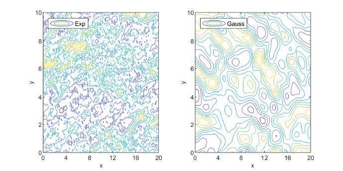
In order to test the numerical methods in conditions of hydraulic conductivity with increasing variability, comparisons are done for log-hydraulic conductivities with exponential and Gaussian correlations. Testing the numerical schemes for these correlation models is highly relevant from the point of view the numerical difficulty of solving the flow problem. Indeed, while a Gaussian correlation ensures the smoothness of the generated hydraulic conductivity samples, in case of exponential correlation the smoothness significantly deteriorates with the increase of the number of modes, the generated samples approaching non-differentiable functions in the limit of an infinite number of modes [72, 74].
The remainder of this paper is organized as follows. Section 2 presents the benchmark problems, the Kraichnan randomization method, and some considerations of the sample-smoothness of the generated hydraulic conductivity fields with Gaussian and exponential correlation. The numerical schemes considered in this study are described in Section 3. The results of the code verification by manufactured solutions are presented in Section 4.1 and the convergence results in Section 4.2. Section 5 presents Monte Carlo inferences and comparisons with first-order theory. Finally, some conclusions of the present study are drawn in Section 6. A presents the computation of the manufactured solutions and B contains tables with estimated order of convergence. Supplementary materials S1–S4 associated with this article are available in the online version.
2 Benchmark flow problems
We consider the two-dimensional steady-state velocity field in saturated porous media with constant porosity determined by the gradient of the hydraulic head according to Darcy’s law [19]
| (1) |
where is an isotropic hydraulic conductivity consisting of a fixed realization of a spatial random function. The velocity solves a conservation equation , which after the substitution of the velocity components (1) gives the following equation for the hydraulic head,
| (2) |
We are looking for numerical solutions of the equations (1)-(2) in a rectangular domain, , subject to boundary conditions given by
| (3) | ||||
| (4) |
where is a constant head.
The hydraulic conductivity fields considered in this study are isotropic, log-normally distributed, with exponential and Gaussian correlations. The random log-hydraulic conductivity field is specified by the ensemble mean , the variance , and the correlation length . The Kraichnan algorithm [40] used to generate samples of fluctuating part of the log-hydraulic conductivity field is a randomized spectral representation of statistically homogeneous Gaussian fields [41]. A general randomization formula, valid for both exponential and Gaussian correlation types, is given by a finite sum of cosine functions,
| (5) |
The probability density of the random vector is given by the Fourier transform of the correlation function of the statistically homogeneous random field divided by the variance and the phases are random numbers uniformly distributed in [42, Eq. (22)].
The smoothness of the field is essentially determined by the correlation of the random field . Sufficient conditions for sample smoothness are given by the existence of higher order derivatives of the correlation function . For instance, in the one-dimensional case, if has a second order derivative at , then the one-dimensional field is equivalent to a field with samples that are continuous with probability one in every finite interval. Moreover, if the fourth derivative exists, is equivalent to a field the sample functions of which have, with probability one, continuous derivatives in every finite interval. These sufficient conditions can hardly be relaxed and one expects that they are very close to the necessary conditions [18, 83].
The smoothness conditions of [18] are fulfilled for instance if the correlation of has a Gaussian shape and is infinitely differentiable, which results in a random field (5) with continuous sample derivatives. A counterexample is the field with an exponential correlation , which is not differentiable at the origin. Since, rigorously speaking, the differentiability of at the origin is only a sufficient condition, we proceed with numerical investigations on the sample-smoothness of the field in case of Gaussian and exponential correlations of the log-hydraulic conductivity with and . The estimations of the spatial derivative of a given realization of the numerically generated one-dimensional field with random modes in (5), computed at , are presented in Figs. 2 and 2. In case of Gaussian correlation the estimations approach the exact value of at obtained by differentiating the expression (22) with fixed. In case of exponential correlation of , the realization of the field apparently approaches a non-differentiable function for , then, by further decreasing one observes a smooth behavior and the approach to the true value of at .
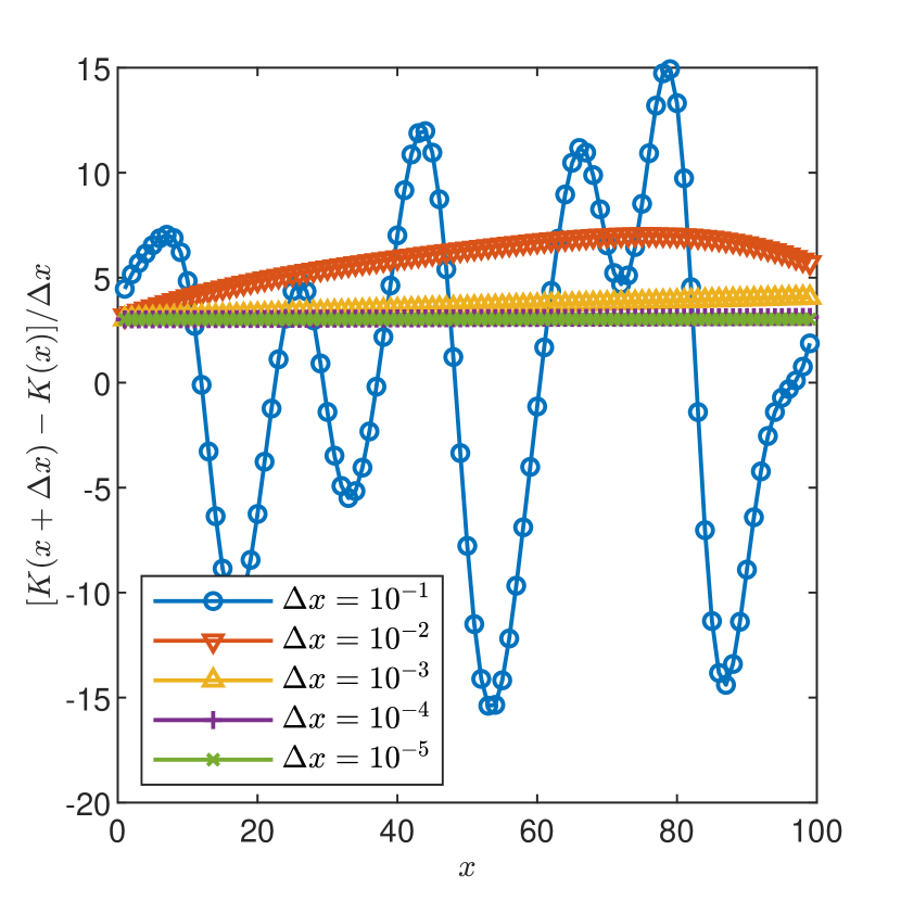
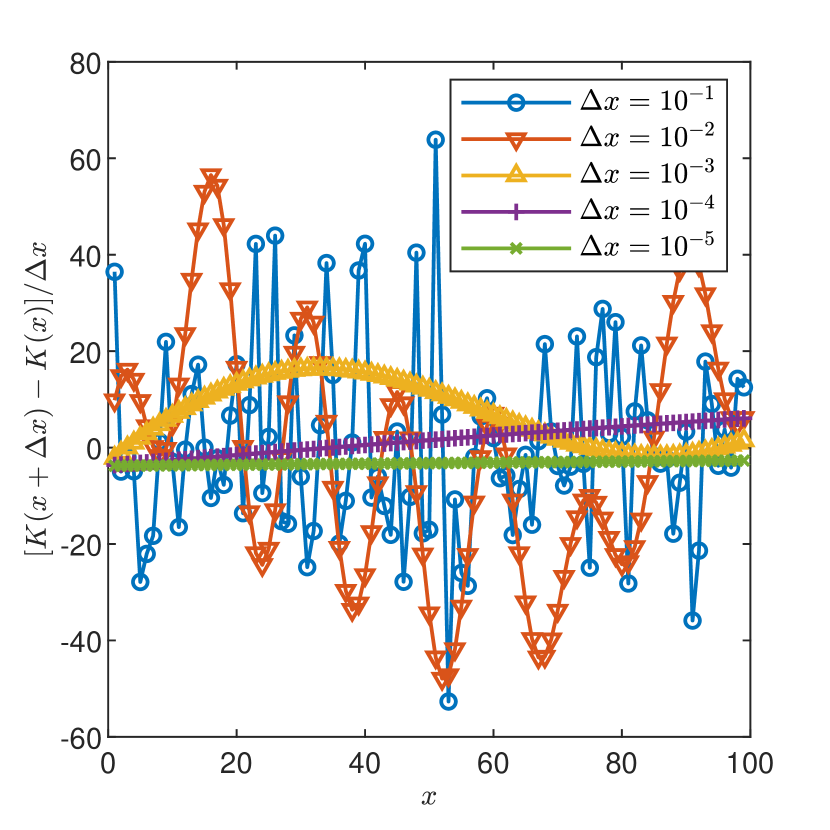
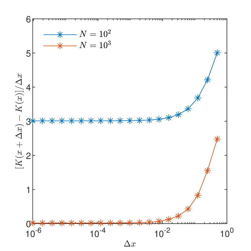
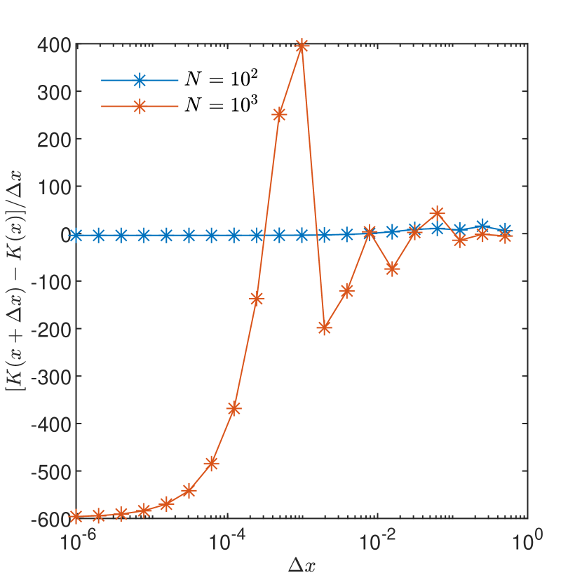
The impact of increasing the number of modes is illustrated by the convergence behavior of the numerical estimates of presented in Figs. 4 and 4. One remarks that while for Gaussian correlation the number of modes has no impact, the convergence towards the exact value of the derivative being practically achieved for , in case of exponential correlation the resolution has to be increased four orders of magnitude () to obtain an accurate approximation of the derivative when increases one order of magnitude.
In order to investigate the robustness and the limits of applicability of the numerical schemes tested in this study, we consider highly oscillating coefficients generated by (5) for isotropic correlations of the random field , , where . As correlation functions, we consider the two extreme cases presented above, i.e., the Gaussian correlation,
| (6) |
which yields analytical samples of , and, respectively, the exponential correlation,
| (7) |
which, in the limit of infinite number of modes , produces non-smooth samples.
To compute the hydraulic conductivity , the geometric mean has to be specified either from experimental data or through its relation with other parameters of the flow problem, such as the mean slope of the hydraulic head, , and the mean velocity . In this study we consider the second approach. According to the boundary conditions (3-4), the mean velocity is aligned to the longitudinal axis . As an input in the field generator, we use a mean hydraulic conductivity related according to Darcy’s law (1) to the mean velocity and the mean slope by . Further, as far as we do not compare velocity fields for different , we generate random conductivity fields by using the relation between the arithmetic and the geometric mean of the log-normal distribution, . The arithmetic mean approximates the effective hydraulic conductivity if [30, 82]. Higher order corrections were also derived as asymptotic approximations for small [24]. But our numerical tests have shown that neither of these corrections is appropriate for statistical inferences, because they lead to underestimations of the mean velocity. Therefore, to compare results obtained with different values of the parameter presented in Section 5, we normalize the velocity components by [see also 42].
The mean hydraulic conductivity is fixed to m/day, a value representative for gravel or coarse sand aquifers [19]. The correlation length in (6) and (7) is set to m and the dimensions of the spatial domain are given in units. In order to compare the results obtained by different schemes for a given realization of the field , the sets of wavenumbers , , and phases are computed with the algorithms for Gaussian and exponential correlation functions described in [42, Sects. 5.2 and 5.3] implemented as C-codes. These coefficients, computed for modes , are stored as data files. Samples of the field are further constructed for the desired numbers of modes and values of the variance , according to (5). The same numerical parameters can be used in either Matlab, C++, or Python codes, to ensure identical values of the fields, in the limit of double precision, irrespective of the programming language. For the purpose of statistical inferences, ensemble of solutions of the flow equations are computed with the same algorithms implemented as functions in each particular scheme.
The longitudinal dimension of the domain, , has to be tens of times larger than (for instance, [1] recommend ). Constrained by considerations of computational tractability, we fix the dimensions of the domain to and . The constant head at the inflow boundary is fixed to . To enable comparisons of the two dimensional solutions obtained with the FDM, FEM, DGM, and GRW numerical schemes tested in the present benchmark, the number of discretization points is set to , in the longitudinal direction, and to in the transverse direction. Consequently, the space steps are fixed at , which, for unit correlation length considered in this study, gives . This value is larger than the resolution of the log-conductivity field usually considered in similar finite difference/element approaches reported in the literature [see e.g., 8, 12, 22, 42]. The fixed resolution considered in this study is appropriate for flow solutions in case of Gaussian correlation of the field but could be to coarse in case of exponential correlation (see Figs.2 – 4).
In case of spectral approaches, the number of collocation points, for both CSM and GSM schemes, is chosen after preliminary tests as large as necessary, possible optimal, to ensure the desired accuracy (see Section 3.4).
The codes based on the numerical schemes considered in this study are first verified by comparisons with manufactured solutions. The approach consists of choosing analytical functions of the dependent variables, , on which one applies the differential operator from the left hand side of Eq. (2), the result being a source term . Hence, is an exact solutions of Eq. (2) with a source term added in the right hand side and modified boundary functions according to the chosen manufactured solution [e.g., 63].
An example of choosing the appropriate manufactured solution for the flow solver within a numerical setting similar to that of the present study can be found in [42, Appendix B]. In order to test the numerical approximations of the differential operators in the flow equation (2), the manufactured solutions used in this study are simple, but not trivial analytical functions with nonzero derivatives up to the highest order of differentiation. The construction of the manufactured solution and of the source term is presented in A. For the purpose of code verification we chose 10 parameter pairs formed with , and the two numbers of modes considered in Figs. 4 and 4, and . A larger set of 21 parameter pairs, also including , , and , has been considered in the extended version of this study [3].
Note that the two values of considered here are relevant for practical applications of the numerical codes. A number of modes of the order is required to obtain accurate simulations of the transport process over tens of correlation scales even for a small variance and a linearized solution of the flow equation [27]. The larger number of modes is needed, in the same conditions, for simulation lengths of hundreds of correlation scales. In the latter case, the small spatial domain considered above can be thought of as a subdomain in a domain decomposition approach. On the other hand, the problem is linear and the correlation of the log-hydraulic conductivity only depends on spatial lags scaled by the correlation length. Thus, the results presented in this benchmark study also can represent solutions to problems with spatial dimensions scaled by the correlation length.
The code verification is completed by convergence tests aiming at comparing the computational order of convergence with the theoretical one. In case of FDM, FEM, DGM, and GRW approaches, computational orders of convergence are estimated by computing error norms of the solutions obtained by successively halving the spatial discretization step with respect to a reference solution obtained with the finest discretization [see e.g. 65, 50]. The approach is different in case of spectral methods, where the convergence is indicated by the decrease towards the round-off plateau of the coefficients of the spectral representation [5]. Convergence tests are performed for and a larger range of variances, .
Validations tests are finally conducted by comparing mean values and variances of the velocity components inferred from ensembles of 100 realizations of the solution of the homogeneous boundary value problem (1-4) for and fixed with theoretical and numerical results given in the literature.
The formulation of the benchmark problems, data files, numerical codes and functions are given in a Git repository [4] which can help the interested readers to test their numerical methods for flows in highly heterogeneous aquifers.
3 Numerical methods
In this section, we describe the methods on which the codes participating in the present benchmark study are based. For the FDM, FEM, and DGM approaches, based on well established finite difference/element methods, only a few aspects relevant for the construction of the numerical scheme will be summarized in the following. The spectral approaches CSM and GSM adapted to this benchmark, as well as the GRW algorithm using computational particles proposed in this article will be presented in more detail.
3.1 Finite difference method
The finite difference method is known to be one of the most feasible and easily implementable numerical methods for partial differential equations [44]. The inhomogeneous version of the flow problem (2-4) for the hydraulic head used in code verification tests consisting of comparisons with manufactured solutions presented in Section 4.1, as well as the homogeneous problem (1-4) used to compute ensembles of velocity fields used for the validation purposes in Section 5 are solved with the FDM of [48]. The method leads to a linear system with a band matrix which is further solved with the mldivide function in our Matlab implementation of the FDM codes.
The codes are based on the following discretization scheme:
| (8) |
where , , represents the data at the grid points and is the value of the numerical solution at the same grid points. In formula (8), we have used the following notations :
| (9) |
3.2 Finite element method
We consider the piecewise affine finite element method (FEM), [see e.g. 38, 69] implemented in FEniCS [2]. The conductivity and the source term are interpolated into finite element spaces as well; for this interpolation we consider piecewise quadratic elements. Better approximations can be obtained by taking higher order finite element spaces for and .
Let us denote by the part of the boundary where Dirichlet conditions are imposed, and by the part of the boundary where Neumann conditions are given.
Consider a Friedrichs–Keller triangulation , where denotes the length of a short side of each isosceles-right triangle. The trial space contains continuous functions that are piecewise affine on each triangle and that satisfy the Dirichlet boundary condition on . The test space consists of continuous piecewise affine functions that vanish on .
For the non-homogeneous equation (2) with right hand side , the linear FEM solves for a trial function such that for any test function the following weak formulation is satisfied:
where is the unit outward normal. The assembled linear system of equations is solved with the default solver in FEniCS, which is the UMFPACK’s Unsymmetric MultiFrontal method.
3.3 Discontinuous Galerkin method
Another method participating in the benchmark is the non-symmetric interior penalty DGM. We consider the same Friedrichs–Keller triangulation as in the previous subsection. Assuming that the test and trial functions are element-wise polynomials of degree at most , element-wise multiplication of Eq. (2) with right hand side by local test functions with support only on , integration over , integration by parts, and selection of suitable numerical fluxes yield the following equation for all that are not adjacent to the domain’s boundary:
Here, denotes the set of faces of , is the unit outward normal with respect to , and is a stabilization parameter. Since the test and trial functions are discontinuous, the numerical fluxes contain averages of functions. The average of a function at a common interface of elements and is (component-wise) given as the arithmetic mean of the traces of this function. The correct way to employ boundary conditions and precise definitions of the corresponding terms can be found in [26, 62, 67]. The following simulations are carried out utilizing piecewise linear test and trial functions, i.e., . The implementation was made using the Matlab/Octave toolbox FESTUNG [29]. The used DGM is known to be of convergence order if the mesh is regular (which holds in our case).
Note that the DGM approach induces significantly larger linear systems of equations than a classical FEM approximation of equal order on the same mesh. This is due to the fact that for DGM schemes, all elements contain three degrees of freedom (DoFs), while for FEM, the corresponding DoFs are shared across element boundaries. This is illustrated in Fig. 5, where a coarse mesh is illustrated: the center point is associated with six DoFs in DGM, while it is associated with a single DoF in a FEM approximation. Hence, the size of the corresponding linear system of equations for DGM is approximately six times the size of the FEM approximation (when neglecting the boundary DoFs where the ratio is only 3:1 and the corner DoFs where the ratio is 2:1 or 1:1). As a consequence, DGM approximations are more costly than FEM approximations when performed on the same mesh, but they also pose some advantages such as local mass conservation, feasibility for local mesh and adaptivity, as well as an intuitive treatment of hanging nodes. The linear systems of equations is solved with Matlab’s direct solver mldivide.
3.4 Spectral methods
As an alternative to finite difference/element methods, we propose in the following the technique of collocation and Galerkin spectral methods in order to solve the one- and two-dimensional flow problems. We refer to [5, 81] for a detailed description of the Chebyshev collocation spectral method. In our implementation of the CSM schemes, we use the explicit analytical expression (22) of the two-dimensional hydraulic conductivity field . For the one-dimensional cases, is obtained by setting in the expression (22) of the two-dimensional field. These allow us to compute the derivatives , , and . To avoid the need to know the analytical expression of the coefficients , we also adapt the algorithm of [70] to construct a GSM approach for one-dimensional flow problems.
3.4.1 Chebyshev collocation spectral methods
We consider for the beginning the one-dimensional problem
| (10) |
where is a source/sink term. Numerical solutions of the problem (10) are computed for a fixed length of the domain of .
For the beginning, we homogenize the problem (10) by using the transformation
| (11) |
Replacing in (10) by (11), one obtains
| (12) |
Further, in order to apply the Chebyshev spectral collocation we use the change of variables to transform the flow problem from to as follows:
| (13) |
where
The flow equation written in matrix form is given by
| (14) |
where and are the first and second order Chebyshev differentiation matrices where we deleted the first and last rows and columns in order to incorporate the boundary conditions. The matrices are generated with chebdif function given in [81]. In the equation (14), are column vectors that contain the values of on the Chebyshev nodes, with the exception of the first and last points.
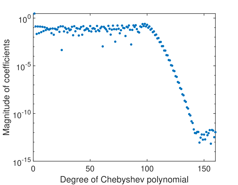
To establish the number of collocation points necessary to obtain the highest accuracy, we first investigate the structure of the numerical solution of the non-homogeneous version of the problem (10) in a scenario with extremely large parameters ( and ), for Gaussian correlation of the field. The source term and the Dirichlet boundary conditions are obtained, similarly to the procedure described in A, for the manufactured solution , . In Fig. 7 we represent the absolute values of the coefficients of the solution’s expansion in the phase space, computed with the fast Chebyshev transform, versus the degree of the Chebyshev polynomial. We observe that for Chebyshev points the coefficients reach the roundoff plateau. Since, due to the accumulation of the truncation errors, large numbers of points could result in an increased error, we also compute the error norm to establish the optimal value of for Gaussian and exponential correlation scenarios. Note that the analysis differs from case to case [see 3, Tables 30 and 31].
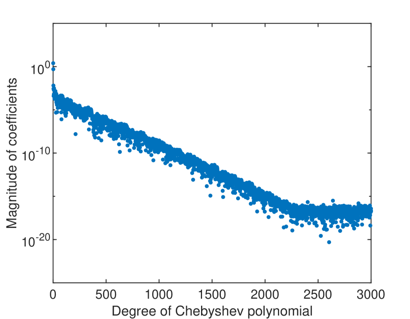
We also investigate the structure of the solution and the convergence for the homogeneous one-dimensional problem ( in (10)) for Gaussian correlation of the field and much smaller parameters, and (see Fig. 7). In absence of an analytical solution of the homogeneous boundary value problem, reaching the roundoff plateau is a guarantee that the numerical solution is highly accurate [5]. We remark that at least collocation points are needed to reach the roundoff plateau of the coefficients. The much larger value of is due to the spatial variability of the homogeneous solution (see Supplementary material S1) which cannot be represented by relatively small , as in case of the simple manufactured solution of the non-homogeneous problem.
In order to apply the Chebyshev collocation method in the two-dimensional case, we reformulate the flow problem (2-4) into the square , similarly to the procedure used in the one-dimensional case, and we transform the boundary conditions by following the approach of [35].
The optimal number of Chebyshev points for the inhomogeneous problem is established, similarly to the one-dimensional case, by increasing from to in both directions and by computing the error for combinations of parameters and in both Gaussian and exponential scenarios [see 3, Tables 34 and 35].
In case of the homogeneous two-dimensional problem, the roundoff plateau is reached with about points in the -direction but a significantly larger number of points would be necessary in the -direction [see 3, Figs. 8 and 9]. Since, according to the discretization scheme (14), the dimension of the problem increases as solving homogeneous two-dimensional problems with CSM schemes requires much larger memory usage than finite difference/element schemes.
3.5 Chebyshev-Galerkin spectral method for one-dimensional flow problems
The flow equation in (10) is a particular case of that considered in the GSM approach of [70],
corresponding to and . The Chebyshev-Galerkin spectral method of [70] will be used in Section 4.1 to solve one-dimensional test problems. Unlike the CSM schemes presented above, the GSM approach avoids the need to compute the derivative of , by using the weak formulation of the problem. The GSM approach, can be applied to more general situations where an analytical form of the field is not available.
3.6 Global random walk method
GRW algorithms solve parabolic partial differential equations by moving computational particles on regular lattices [73, 74, 80]. Solutions of the elliptic equation for the hydraulic head with time independent boundary conditions can be obtained by solving the associated nonstationary equation with GRW algorithms on staggered grids (C. Vamoş, 2016, unpublished). Following this idea, we look for a solution of the flow equation (2) with a source term in the right-hand side given by the steady-state limit of the solution of the explicit staggered finite difference scheme
| (15) |
where is a constant equal to a unit length.
The field of hydraulic head is further approximated with a system of random walkers on the regular lattice of the finite difference scheme as . Considering in (3.6) , as in Section 2, the hydraulic conductivity, the time step , and the space step are related by the dimensionless parameter
| (16) |
With these, the staggered scheme (3.6) becomes
| (17) | |||||
where the source term is approximated by using the floor function . The contributions to lattice sites from neighboring sites summed up in (17) are obtained with the GRW algorithm which moves particles from sites to first-neighbor sites according to
| (18) | |||||
For consistency with the (17), the stochastic averages of the quantities in (18) verify
| (19) |
The parameters defined by (16) are jump probabilities which, as follows from (3.6), are restricted by .
The terms in (18) are binomial random variables. They are efficiently approximated by applying the relation for averages, (3.6), to the actual numbers of particles at lattice sites. Next, the reminders of multiplication by and of the floor function applied to are summed up and a particle is allocated to the lattice site where the sum of reminders reaches the unity [see 74, Sect. 3.3.2.2].
Giving up the particle indivisibility and representing by real numbers, one obtains a deterministic GRW algorithm, where the numbers of particles jumping to neighbor sites or remaining at the same site are exactly given by the relations (3.6) without average. Preliminary tests indicate that the GRW algorithm with particles requires fewer time iterations to reach the steady state, but the deterministic version, which preforms fewer arithmetical operations per iteration step, is overall faster. Therefore, in the following we use the deterministic GRW algorithm implemented in Matlab or C++ codes.
To solve the flow equation by the GRW algorithm (16-3.6), the boundary conditions (3) and (4) have to be completed by appropriate initial conditions. The homogeneous problem () is solved for an initial condition given by the mean slope of the pressure head (determined by the Dirichlet boundary conditions). For comparison with analytical manufactured solutions, the inhomogeneous problem () is solved for an initial condition given be the analytical solution itself.
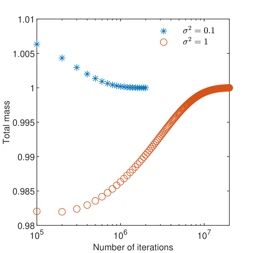
For an arbitrary initial condition, one obtains a transitory, non-stationary GRW solution which approaches the stationary solution after a number of time iterations depending on the level of difficulty of the particular problem. The steady state is indicated by a constant number of particles or, in case of deterministic GRW, by the “total mass” defined as integral of the solution over the lattice, normalized by the final mass, as illustrated in Figs. 9 and 9 for different solutions of the homogeneous problem.
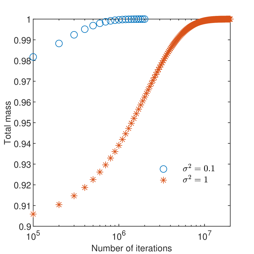
The iterations needed to obtain stationary solutions require considerably large computing time (from 10 minutes for iterations to 2.5 hours for iterations). Faster computations can be designed by using a domain decomposition parallelization of each iteration.
Most of the computations were carried out with a Matlab implementation of the GRW code. For the comparisons with manufactured solutions in case of exponential correlation of the field, which take very long time, we use an executable mex-function of a C++ implementation of the flow solver. This procedure speeds up the computation by a factor of 1.5.
4 Benchmark tests
4.1 Code verification by manufactured solutions
The non-homogeneous problem problem, (2-4) with source term given by (23) and modified Dirichlet and Neumann boundary conditions (21), is solved on the two-dimensional domain described in Section 2. The problem is parameterized by using the sets of wavenumbers and phases for a fixed realizations of the field stored in the Git repository FlowBenchmark [4]. The FDM, FEM, DGM, and GRW schemes are constructed on uniform grids with step sizes , in all cases excepting those of GRW solutions for Gaussian correlation where , and the errors of the numerical solutions with respect to the manufactured solution given by (20) are quantified by the discrete norm. The CSM solutions are computed for the optimal number of Chebyshev points identified by preliminary tests as explained in Section 3.4.1 above and the errors at collocation points are quantified by the vector norm. The code verification results for the two values of and increasing variances of the field are presented in Tables 1-4.
| 0.1 | 1 | 2 | 4 | 6 | |
|---|---|---|---|---|---|
| FDM | 1.03e-03 | 2.00e-03 | 7.95e-03 | 4.34e-02 | 1.45e-01 |
| FEM | 1.61e-03 | 2.97e-03 | 3.93e-03 | 5.60e-03 | 7.06e-03 |
| DGM | 1.11e-03 | 1.15e-03 | 1.41e-03 | 2.10e-03 | 2.76e-03 |
| CSM | 3.58e-13 | 6.75e-13 | 9.00e-12 | 1.06e-10 | 6.54e-10 |
| GRW | 3.16e-02 | 4.80e-02 | 1.35e-01 | – | – |
| 0.1 | 1 | 2 | 4 | 6 | |
|---|---|---|---|---|---|
| FDM | 1.09e-03 | 8.91e-03 | 4.23e-02 | 3.65e-01 | 1.88e+00 |
| FEM | 2.17e-03 | 5.60e-03 | 7.60e-03 | 1.01e-02 | 1.16e-02 |
| DGM | 1.11e-03 | 1.19e-03 | 1.41e-03 | 1.84e-03 | 2.29e-03 |
| CSM | 3.71e-13 | 4.50e-12 | 1.25e-11 | 2.50e-10 | 2.23e-09 |
| GRW | 6.81e-02 | 5.59e-01 | 1.78e+00 | – | – |
| 0.1 | 1 | 2 | 4 | 6 | |
|---|---|---|---|---|---|
| FDM | 1.17e-01 | 2.60e+00 | 3.61e+00 | 9.41e+01 | 7.15e+02 |
| FEM | 9.08e-03 | 5.07e-01 | 3.57e+00 | 4.28e+01 | 2.41e+02 |
| DGM | 4.58e-02 | 2.59e-01 | 5.31e-01 | 2.91e+00 | 1.53e+01 |
| CSM | 8.11e-12 | 2.15e-11 | 7.24e-11 | 3.58e-10 | 1.00e-09 |
| GRW | 9.45e-02 | 7.57e-01 | 1.64e+00 | – | – |
| 0.1 | 1 | 2 | 4 | 6 | |
|---|---|---|---|---|---|
| FDM | 3.58e-02 | 3.09e+00 | 1.42e+01 | 9.79e+01 | 1.45e+03 |
| FEM | 1.29e-02 | 8.46e-01 | 3.66e+00 | 4.87e+01 | 6.06e+02 |
| DGM | 1.37e-02 | 1.72e-01 | 1.20e+00 | 1.32e+01 | 6.87e+01 |
| CSM | 1.63e-11 | 3.42e-11 | 3.38e-11 | 2.47e-10 | 1.67e-09 |
| GRW | 1.13e-01 | 1.28e+00 | 4.12e+00 | – | – |
As shown in Table 1, all the methods solve the test problems in the Gaussian cases with with a good, or at least an acceptable accuracy. The increase of the number of modes to (Table 2) affects the accuracy of the FDM and GRW schemes, which produce errors larger that one (i.e., from the maximum value of the manufactured solution (20)) for (FDM) and (GRW). There are also significant differences among the methods. The accuracy of the DGM scheme is one and two orders of magnitude better than that of the FDM and FEM schemes and the precision of the CSM scheme is close to the roundoff plateau. The GRW solutions, computed on a coarser grid, are still accurate up to and . Since the time needed to reach steady-state GRW solutions ranges from a few minutes to a couple of hors, for the cases shown in these tables, the cases with were not investigated with the GRW method.
For exponential correlation of the field, excepting CSM, the accuracy of all the other schemes is affected by the increase of and (Tables 3 and 4). For the FDM and the FEM schemes, the errors become larger than one for with and , respectively, and take huge values of the order and , respectively, for and . Accurate DGM solutions are realizable for in case and for in case . For the same resolution of the grid (), stationary GRW solutions in exponential cases can be obtained after considerable large numbers of iterations from to more than , which require computing times from hours to days. Note that in the cases with and the GRW solutions are not yet strictly stationary and the corresponding values have to be regarded as lower bound errors. In these circumstances, accurate GRW solutions are feasible for and or for and .
The extremely small errors of the CSM solutions should not be surprising. For a fixed realization of the random field , the coefficients and their derivatives used in the CSM schemes are analytical functions (see Section 3.4.1). The source function (23) is an analytical function as well. Since all these functions are evaluated at the collocation points with the machine precision, the only source of errors can be the limited number of points used to represent the solution. This number is relatively small in case of the smooth analytical solution (23). If the same problem is solved with the GSM scheme, which does not use the derivative of the coefficients, a much larger number of points is needed to resolve the structure of the and fields. This situation is illustrated by the comparison of the CSM and GSM errors in Table 5 which shows that accurate GSM solutions are obtained by increasing the density of the collocation points by one order of magnitude in case of Gaussian correlation of the field, and by two orders of magnitude in the exponential case.
| 0.1 | 1 | 2 | 4 | 6 | |
|---|---|---|---|---|---|
| CSM | 1.11e-13 | 1.03e-13 | 1.99e-13 | 6.50e-13 | 1.88e-12 |
| GSM1 | 8.87e-12 | 3.46e-11 | 2.45e-10 | 1.81e-09 | 1.11e-08 |
| GSM2 | 2.55e+02 | 5.75e+03 | 3.70e+04 | 4.17e+05 | 3.01e+06 |
| GSM3 | 5.43e-11 | 3.12e-08 | 1.01e-06 | 4.55e-05 | 4.46e-04 |
4.2 Estimated order of convergence
Numerically estimated orders of convergence (EOC) of the FDM, FEM, DGM, and GRW schemes for combinations of parameters and are presented in B. They are computed from numerical solutions of the homogeneous problem obtained for successive refinements of the grid according to formula 24. For the non-stationary GRW scheme, the EOC values are computed from solutions on refined grids after the first temporal iteration.
In the Gaussian case, the EOC values are close to the theoretical convergence order 2 for all schemes (see Tables 1, 3, 5, and 7). The situation is different in case of exponential correlation of the field. The results for the FDM scheme presented in Table 2 show an irregular behavior of the EOC values, negative values corresponding to non-monotonous decrease of the error, and the lack of a general decreasing trend of the errors for almost all combinations of and . For the other three schemes there are no negative EOC values but the order of convergence deteriorates to or in most cases (see Tables 4, 6, and 8). Hence, the convergence behavior is strongly influenced by the shape of the correlation function but there is no evidence for a dependence on and .
The convergence of the CSM scheme can be assessed indirectly by verifying the behavior of the Chebyshev coefficients. As we have seen in Section 3.4.1, the convergence of the CSM scheme for homogeneous problems requires much larger numbers of collocation points than in the inhomogeneous cases. With the maximum number of 160 points on both spatial directions permitted by the computational constraints, the solutions for and are accurate enough to be used in Monte Carlo simulations only for Gaussian correlation of the field. With the same parameters and exponential correlation function, the CSM scheme may produce quite inaccurate solutions for some realizations of the field (see Section 5 below).
5 Statistical inferences
Ensembles of numerical solutions of the flow problem are often used for the purpose of validation of the numerical schemes through comparisons with first-order approximation results (e.g., [7, 22, 68, 71]). The latter are obtained by perturbation expansions truncated at the first order in , equivalent to a linearization of the flow problem (1-4) (e.g., [19, 31]). Here, we consider first-order approximations of the velocity field numerically generated with a Kraichnan procedure, based on proportionality of the spectral densities of the random velocity and that of the field [78, Appendix A]. The number of random periodic modes used in the Kraichnan generators of the hydraulic conductivity and of the velocity field (in the case of the linear approximation) is set to . Validation tests of the five schemes are performed for fields with Gaussian and exponential correlations and a fixed small variance . The deviation from the predictions of the linear approximation is further investigated with the FDM, FEM, DGM, and GRW schemes for increasing of 0.5, 1, 1.5, and 2. The number of realizations, in all cases investigated here, is fixed to . Numerical investigations indicate that the chosen values of the parameters and ensure unbiased statistical estimations of the dispersion of a passive scalar transported over tens of correlation lengths in heterogeneous aquifers characterized by a small variance of the field [27].
The homogenous problem (1-4) is solved in the same two-dimensional domain, with and , as that used for code verification tests in the previous section. Graphical illustrations and analysis of numerical solutions are given in Supplementary materials S1 to S4. The ensemble of realizations were computed for space steps , with the FDM scheme and, to reduce the computational effort, for larger steps , with the FEM and DGM schemes, and , with the GRW scheme. Constrained by the maximum Matlab array size allowed on the computer used to obtain CSM solutions, we use a limited number of 160 Chebyshev collocation points in both - and -directions, even though a larger number of points in -direction is required to obtain accurate solutions [see 3, Fig. 9]. Sample solutions obtained with FDM are illustrated in Supplementary material S1. FEM, DGM, and GRW solutions, not shown in S1, have a similar appearance. Instead, among the realizations of the CSM solution for exponential correlation of the field there also are unacceptable solutions with extremely large and irregular variations. Therefore, we selected an ensemble of 100 valid realizations by disregarding the “bad” solutions after the visual inspection of the larger initial ensemble of solutions, as illustrated in Supplementary material S2. The issue of “bad realizations” is common in situations where, due to computational constraints, numerical simulations have to be conducted on relatively coarse grids (we already encountered this issue during the preparation of the transport simulations presented in [57, 76]).
Monte Carlo inferences of the mean and variance are obtained by computing averages over the ensembles of realizations followed by spatial averages [75, Appendix B3]. Error bounds of the ensemble-space averages are given by standard deviations of the ensemble averages at grid points, estimated by spatial averages. The spatial averaging domain is an inner region of the computational domain unaffected by the boundary conditions approximately delimited by visual inspection of the variances estimated on longitudinal and transverse sections through the computation domain presented in Supplementary materials S3 and S4 [see also 7, 42].
Theoretical investigations indicate that the variance of the hydraulic head is much smaller than that of the hydraulic conductivity. Spectral perturbation approaches for flow in two- and three-dimensions predict variances of the order [1, 6, 52]. The estimated variances presented in Table 6 show an acceptable agreement with the spectral theory, which for our numerical parameters predict .
The first-order approximate relations between the variance of the velocity components, and , and the variance of the field are given by and , respectively [19, Eq. (3.7.27)]. Note that these relations do not depend on the shape of the correlation function of the field. Since, as mentioned in Section 2, for the purpose of statistical inferences we use dimensionless velocities, . Then, with the smallest variance of the field considered in this study, , the velocity variances predicted by the linear theory are and , respectively.
The estimated mean values and variances of the velocity components are presented in Tables 7 and 8. FDM, FEM, DGM, and GRW results are generally close to theoretical first-order predictions within a range of less than 10% in case of FDM, FEM, DGM, and GRW approaches, excepting FEM estimated variance of the transverse velocity in the Gaussian case which deviates with about 30%. CSM results show deviations of about 30%, for the variance of the transverse velocity in the Gaussian case, and deviations even larger than 100% for both velocity variances, in the exponential case. These differences can be again attributed to the limited number of collocation points used in the CSM approach.
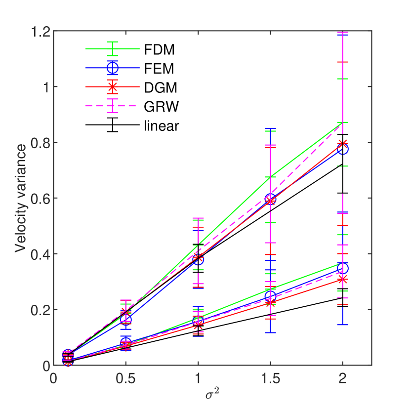
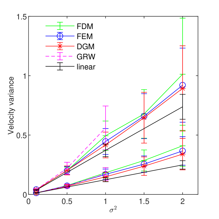
The results obtained with the FDM, FEM, DGM, and GRW approaches for larger are shown in Figs. 11 and 11. We remark that the velocity variances progressively increase above the trend predicted by the linear theory, similarly to the Monte Carlo results presented in the literature (e.g., [7, 42, 68]). The differences between the results obtained with the three methods remain within the estimated error bounds determined by the present numerical setup (number of realizations, resolution, and dimension of the computational domain). For the estimated variances practically coincide with the first-order predictions. Within this range, velocity fields can be quite well approximated by the linearized solution of the flow problem and simulations of solute transport in groundwater can be carried out with Kraichnan generated velocity fields at lower computational costs [75, 73, 78].
We conclude this section with a remark about the GRW results. The ensembles of GRW simulations were computed for iterations in all cases, excepting the Gaussian case with , where the number of iterations was set to . As indicated by Figs. 9 and 9, as well as by Supplementary materials S3 and S4, these numbers of iterations are not large enough to ensure the convergence of the solution for homogeneous problems. Surprisingly, the variance estimates from Tables 7-8 deviate with maximum 10% from the predictions of the first order theory for small . For larger , the GRW results are also close to those obtained with the FDM, FEM, and DGM schemes for in Gaussian case (Fig. 11) and for in exponential case (Fig. 11).
| Gaussian correlation | Exponential correlation | |
|---|---|---|
| FDM | 3.47e-04 3.77e-05 | 5.91e-04 5.79e-05 |
| FEM | 6.05e-04 1.06e-04 | 5.52e-04 8.45e-05 |
| DGM | 2.48e-04 1.12e-04 | 4.69e-04 2.44e-04 |
| CSM | 2.07e-04 1.46e-04 | 5.64e-04 4.57e-04 |
| GRW | 3.81e-04 6.06e-05 | 5.69e-04 1.08e-04 |
| linear | 1.00 2.07e-02 | 1.56e-03 1.13e-02 | 3.75e-02 4.96e-03 | 1.27e-02 1.61e-03 |
|---|---|---|---|---|
| FDM | 1.01 1.08e-01 | -5.32e-03 8.37e-03 | 3.66e-02 4.52e-03 | 1.34e-02 1.22e-03 |
| FEM | 1.00 2.13e-02 | -1.05e-02 1.49e-02 | 3.70e-02 4.51e-03 | 1.67e-02 2.94e-03 |
| DGM | 1.01 9.40e-02 | -3.20e-03 9.80e-03 | 3.76e-02 5.91e-03 | 1.32e-02 1.73e-03 |
| CSM | 1.00 2.27e-02 | 4.46e-04 9.17e-03 | 3.96e-02 9.11e-03 | 8.03e-03 5.36e-03 |
| GRW | 1.00 1.96e-02 | -9.19e-04 1.21e-02 | 4.14e-02 6.80e-03 | 1.38e-02 3.00e-03 |
| linear | 0.99 1.81e-02 | 2.60e-03 1.04e-02 | 3.66e-02 5.17e-03 | 1.25e-02 1.78e-03 |
|---|---|---|---|---|
| FDM | 1.00 1.06e-01 | 2.20e-04 1.03e-02 | 3.97e-02 4.04e-03 | 1.27e-02 8.97e-04 |
| FEM | 1.00 1.56e-02 | 7.26e-04 9.46e-03 | 4.14e-02 6.48e-03 | 1.25e-02 2.05e-03 |
| DGM | 1.01 9.35e-02 | 1.66e-03 1.10e-02 | 3.96e-02 4.71e-03 | 1.30e-02 1.86e-03 |
| CSM | 0.99 3.07e-02 | 1.63e-03 1.83e-02 | 8.65e-02 4.17e-02 | 3.61e-02 2.55e-02 |
| GRW | 1.00 2.00e-02 | -1.60e-03 1.09e-02 | 4.08e-02 6.70e-03 | 1.19e-02 1.80e-03 |
6 Discussion and conclusions
The numerical approaches tested in the present benchmark study passed, at least partially, the validation test consisting of comparisons of the numerical solutions obtained for and with theoretical results provided by first-order perturbation approaches. For larger variances, up to , the statistical inferences performed by averaging over Monte Carlo ensembles of solutions given by the FDM, FEM, DGM, and GRW schemes were close to those obtained by simulations with similar numerical setup reported in the literature. However, these encouraging results are not a guarantee for the accuracy of the numerical method in case of higher values of and , needed to solve the flow problem for highly heterogeneous aquifers and large spatial scales. This is indicated, for instance, by the situation of the GRW ensembles of solutions for Gaussian correlation of the field which provide satisfactory statistical estimates even though they are not yet convergent (see Section 5) and cannot be used for single-realization approaches in subsurface hydrology.
For Gaussian correlation of the field the code verification tests were accurately solved, with the exception of the FDM solution for and and that of the GRW solutions for and . Instead, in case of exponential correlation, for all the schemes, excepting the CSM scheme, there are ranges of parameters for which accurate solutions are not realizable: for FDM, for FEM, and for DGM, and for GRW. The limited solvability of the flow problem in case of exponential correlation found in our benchmark study, for a resolution of the numerical solution which is one order of magnitude higher than usually recommended [see e.g., 1, 22], completes similar results presented in the literature. For instance, [12] report difficulties to obtain the convergence of their numerical schemes for exponential correlation of the field with and [33] show that for high resolution of the exponentially correlated field with the required discretization of the hydraulic head solution exceeds the limit of the available computing resources.
The observed large errors produced by the three related discretization schemes, FDM, FEM, and DGM, in the test scenarios with exponential correlation and large values of the parameters and (cf. Tables 3 and 4) may be explained as follows: The listed errors consist of the discretization error of the respective numerical scheme and the error of the linear solver. In practice, the latter one cannot be computed, however, the observed high condition numbers and the computed residuals indicate that the error of the linear solver grows when using the above-mentioned parameters (in fact, the product of condition number and residual is an upper bound for the arithmetic error [37]). More precisely, we found that the condition number increases with in a comparable way for both Gaussian and exponential correlation models and for both numbers of modes. The residuals remain almost unchanged in the Gaussian case, but in exponential case, the increase of and cause the increase of the residuals and, consequently, the increase of the error bound [3, Sect. 9]. Regarding the linear solver: for the FDM and DGM schemes we used Matlab’s direct solver mldivide, which for our system matrices, calls UMFPACK’s Unsymmetric MultiFrontal method [20], and for the FEniCS implementation of the FEM scheme we used the default solver in FEniCS, which calls UMFPACK as well. We also tested various other solvers (e.g., UMFPACK’s SPQR [21] and ILUPACK’s AMG_solver [10]), however, a smaller residual was not producible.
In exponential cases of large and , the coefficients contain large numbers of periodic modes with amplitudes spanning over several orders of magnitude. The high resolution necessary to prevent the occurrence of ill-conditioned matrices and large residuals leads to extremely large degrees of freedom of the linear system of equations which render impractical, from the point of view of computational resources, the use of direct flow solvers such as FDM, FEM, and DGM considered in this study. A possible remedy could be provided by numerical upscaling techniques developed for problems with rough coefficients, which capture the effect of small scales on large scales without resolving the small scale details [13, 36, 39].
CSM schemes verify the manufactured analytical solutions with extremely small errors in both one- and two-dimensional cases. This high precision is rendered possible by the use of the analytical expressions of the derivatives of the field given by the Kraichnan algorithm. The convergence is demonstrated by the decrease of Chebyshev coefficients towards the roundoff plateau. The non-homogeneous flow problem can be solved with relatively small numbers of collocation points (less than 100 points on both spatial directions), which are enough for the spectral representation of the simple, smooth manufactured solutions chosen for the purpose of code verification. But in case of highly oscillating solutions of the homogeneous problem for exponential correlation of the field, a much larger number of points is required, which increases the dimension of the problem beyond the limit of the available memory. Due to this constraint, the maximum number of collocation points in each direction has been fixed to 160, which did not ensure reliable solutions for all the realizations of .
The GSM scheme has been proposed to avoid the use of the analytical derivative of the hydraulic conductivity and has been used only in solving the one-dimensional non-homogeneous problem for comparisons with manufactured solutions. The errors are again very small in the Gaussian case, but extremely large in the exponential case. Some tests made in the attempt to improve the precision indicate that exceedingly large computing resources would be necessary to render the problem computationally feasible (see Table 5).
The GRW scheme is a transitory scheme using computational particles, which is accurate and unconditionally stable. The drawback is the large number of time iterations needed to reach the stationary state corresponding to the steady-state solution of the flow problem. In the Gaussian case, approximations with satisfactory accuracy of the manufactured solution can be obtained with a coarse discretization in reasonable computing times from minutes to hours. In the exponential case, a much finer discretization is needed and the computing time increases from hours to days.
The numerical schemes tested so far on benchmark problems have their own strengths which make them useful in specific applications, depending on the objective pursued. FDM schemes are appropriate for fast computations of Monte Carlo ensembles in case of moderate aquifer heterogeneity, FEM and DGM schemes are appropriate to cope with higher heterogeneity in either single-realization or Monte Carlo approaches, GRW is rather appropriate for single-realization flow problems with heterogeneous coefficients, and CSM/GSM approaches could be useful in solving problems with heterogeneous coefficients and source terms given by smooth functions. We have seen that all the schemes tested in this study face the issue of computational feasibility in case of an exponential structure of the log-conductivity field. It is therefore recommendable that, unless well documented by experimental data for a specific problem, the exponential correlation model should be avoided. Instead, Gaussian models can be used to account for effective dispersion associated with an integral scale [19, 79], as well as in flow and transport simulations for fractal aquifer structures [e.g., 25].
Acknowledgements
The authors are grateful to Dr. Maria Crăciun, for her help in testing the random field generators, and to Dr. Emil Cătinaş for carefully reading the manuscript. Andreas Rupp acknowledges the financial support of the Deutsche Forschungsgemeinschaft (DFG) – Germany under Grants RU 2179 “MAD Soil - Microaggregates: Formation and turnover of the structural building blocks of soils” and EXC 2181 “STRUCTURES: A unifying approach to emergent phenomena in the physical world, mathematics, and complex data”. The work of Nicolae Suciu was supported by the DFG Grant SU 415/4-1 “Integrated global random walk model for reactive transport in groundwater adapted to measurement spatio-temporal scales”.
Appendix A Manufactured solutions
We consider the following smooth manufactured solution :
| (20) |
along with the Dirichlet and Neumann boundary conditions :
| (21) |
The function is given by
| (22) |
where we use the shorthand notations and .
Appendix B Estimated order of convergence
The convergence of the numerical schemes is investigated numerically by solving the homogeneous problem (2-4) for successive refinements of the grid [see e.g., 50]. The hydraulic conductivity fields are computed for each pair of parameters and with the same sets of wavenumbers and phases as those used above for the code verification procedure in Section 4.1.
We start with and obtain refinements of the grid by successively halving the space steps up to , in case of FDM and GRW schemes, and with refinements from to for FEM and DGM schemes. The corresponding solutions are denoted by , . The estimated order of convergence that describes the decrease in logarithmic scale of the error, quantified by the vector norm , is computed according to
| (24) |
| EOC | EOC | EOC | EOC | |||||||
|---|---|---|---|---|---|---|---|---|---|---|
| 2.28e-3 | 2.00 | 5.71e-4 | 2.02 | 1.41e-4 | 2.07 | 3.36e-5 | 2.32 | 6.72e-6 | ||
| 3.03e-2 | 1.98 | 7.68e-3 | 2.01 | 1.90e-3 | 2.07 | 4.54e-4 | 2.32 | 9.09e-5 | ||
| 4.10e-2 | 1.98 | 1.04e-2 | 2.01 | 2.58e-3 | 2.07 | 6.16e-4 | 2.32 | 1.23e-4 | ||
| 4.92e-3 | 2.00 | 1.23e-3 | 2.02 | 3.04e-4 | 2.07 | 7.24e-5 | 2.32 | 1.45e-5 | ||
| 1.43e-1 | 1.99 | 3.59e-2 | 2.01 | 8.90e-3 | 2.07 | 2.12e-3 | 2.32 | 4.24e-4 | ||
| 3.58e-1 | 1.98 | 9.09e-2 | 2.00 | 2.26e-2 | 2.07 | 5.38e-3 | 2.32 | 1.08e-3 |
| EOC | EOC | EOC | EOC | |||||||
|---|---|---|---|---|---|---|---|---|---|---|
| 1.00e-2 | 0.00 | 1.00e-2 | 2.27 | 2.07e-3 | -1.75 | 6.95e-3 | 0.30 | 5.65e-3 | ||
| 1.06e+0 | 1.14 | 4.82e-1 | 0.72 | 2.93e-1 | 0.72 | 1.78e-1 | 0.25 | 1.50e-1 | ||
| 2.80e+0 | 1.47 | 1.01e+0 | 0.46 | 7.33e-1 | 1.18 | 3.24e-1 | 0.12 | 2.98e-1 | ||
| 9.31e-3 | 1.47 | 3.36e-3 | 1.01 | 1.67e-3 | 0.59 | 1.11e-3 | 0.38 | 8.52e-4 | ||
| 1.45e-1 | 0.08 | 1.37e-1 | 0.40 | 1.04e-1 | 0.59 | 6.89e-2 | 2.14 | 1.56e-2 | ||
| 2.64e-1 | -1.30 | 6.49e-1 | 0.60 | 4.28e-1 | 0.41 | 3.23e-1 | 2.98 | 4.09e-2 |
| EOC | EOC | EOC | EOC | |||||||
|---|---|---|---|---|---|---|---|---|---|---|
| 5.02e-3 | 1.94 | 1.30e-3 | 1.99 | 3.27e-4 | 2.05 | 7.85e-5 | 2.28 | 1.61e-5 | ||
| 6.30e-2 | 1.98 | 1.58e-2 | 2.01 | 3.93e-3 | 2.06 | 9.395e-4 | 2.30 | 1.90e-4 | ||
| 1.48e-1 | 2.04 | 3.60e-2 | 2.03 | 8.81e-3 | 2.06 | 2.10e-3 | 2.30 | 4.25e-4 | ||
| 5.96e-3 | 1.90 | 1.59e-3 | 1.99 | 4.00e-4 | 2.05 | 9.61e-5 | 2.28 | 1.96e-5 | ||
| 7.59e-2 | 1.90 | 0.02e-2 | 2.00 | 5.05e-3 | 2.06 | 1.20e-3 | 2.30 | 2.45e-4 | ||
| 1.62e-1 | 2.04 | 3.95e-2 | 2.04 | 9.57e-3 | 2.07 | 2.27e-3 | 2.30 | 4.62e-4 |
| EOC | EOC | EOC | EOC | |||||||
|---|---|---|---|---|---|---|---|---|---|---|
| 8.88e-3 | 1.38 | 3.39e-3 | 1.26 | 1.40e-3 | 1.43 | 5.22e-4 | 1.73 | 1.57e-4 | ||
| 1.95e-1 | 1.78 | 5.65e-2 | 1.01 | 2.79e-2 | 0.84 | 1.55e-2 | 1.59 | 5.16e-3 | ||
| 4.38e-1 | 1.86 | 1.19e-1 | 0.74 | 7.15e-2 | 0.65 | 4.54e-2 | 1.53 | 1.57e-2 | ||
| 1.40e-2 | 1.76 | 4.14e-3 | 1.53 | 1.43e-3 | 1.45 | 5.22e-4 | 2.09 | 1.21e-4 | ||
| 2.09e-1 | 1.89 | 5.64e-2 | 1.41 | 2.10e-2 | 1.20 | 9.16e-3 | 1.90 | 2.44e-3 | ||
| 5.03e-1 | 2.12 | 1.11e-1 | 1.39 | 4.38e-2 | 1.20 | 1.89e-2 | 1.83 | 5.32e-3 |
| EOC | EOC | EOC | EOC | |||||||
|---|---|---|---|---|---|---|---|---|---|---|
| 7.43e-3 | 2.02 | 1.83e-3 | 2.01 | 4.52e-4 | 1.92 | 1.19e-4 | 1.34 | 4.69e-5 | ||
| 1.27e-1 | 2.00 | 3.16e-2 | 2.02 | 7.74e-3 | 2.08 | 1.83e-3 | 2.31 | 3.69e-4 | ||
| 1.57e-1 | 2.03 | 3.83e-2 | 2.01 | 9.50e-3 | 2.07 | 2.26e-3 | 2.30 | 4.56e-4 | ||
| 8.15e-3 | 2.10 | 1.89e-3 | 2.07 | 4.49e-4 | 1.94 | 1.17e-4 | 1.39 | 4.45e-5 | ||
| 7.53e-2 | 2.09 | 1.76e-2 | 2.07 | 4.18e-3 | 2.10 | 9.74e-4 | 2.29 | 1.99e-4 | ||
| 2.76e-1 | 2.07 | 6.55e-2 | 2.05 | 1.58e-2 | 2.08 | 3.73e-3 | 2.31 | 7.48e-4 |
| EOC | EOC | EOC | EOC | |||||||
|---|---|---|---|---|---|---|---|---|---|---|
| 2.17e-2 | 1.02 | 1.07e-2 | 1.85 | 2.96e-3 | 1.69 | 9.16e-4 | 0.14 | 8.29e-4 | ||
| 2.35e-1 | 0.86 | 1.29e-1 | 0.84 | 7.19e-2 | 1.10 | 3.34e-2 | 1.60 | 1.10e-2 | ||
| 2.56e-1 | 1.57 | 8.59e-2 | 0.12 | 7.86e-2 | 0.74 | 4.68e-2 | 1.71 | 1.43e-2 | ||
| 2.32e-2 | 1.42 | 8.66e-3 | 1.74 | 2.58e-3 | 1.35 | 1.01e-3 | 1.90 | 2.70e-4 | ||
| 1.83e-1 | 1.01 | 9.03e-2 | 0.84 | 5.02e-2 | 1.29 | 2.04e-2 | 1.33 | 8.07e-3 | ||
| 5.03e-1 | 2.27 | 1.04e-1 | 1.09 | 4.88e-2 | 1.02 | 2.39e-2 | 1.03 | 1.17e-2 |
| EOC | EOC | EOC | EOC | |||||||
|---|---|---|---|---|---|---|---|---|---|---|
| 2.80e-04 | 2.01 | 6.97e-05 | 2.02 | 1.72e-05 | 2.07 | 4.10e-06 | 2.32 | 8.20e-07 | ||
| 2.78e-04 | 2.00 | 6.93e-05 | 2.02 | 1.71e-05 | 2.07 | 4.08e-06 | 2.32 | 8.15e-07 | ||
| 2.84e-04 | 2.01 | 7.07e-05 | 2.01 | 1.75e-05 | 2.07 | 4.16e-06 | 2.32 | 8.32e-07 | ||
| 2.91e-04 | 2.01 | 7.25e-05 | 2.02 | 1.79e-05 | 2.07 | 4.27e-06 | 2.32 | 8.53e-07 | ||
| 2.66e-04 | 2.00 | 6.63e-05 | 2.02 | 1.64e-05 | 2.07 | 3.90e-06 | 2.32 | 7.79e-07 | ||
| 2.64e-04 | 2.00 | 6.58e-05 | 2.02 | 1.62e-05 | 2.07 | 3.87e-06 | 2.32 | 7.73e-07 |
| EOC | EOC | EOC | EOC | |||||||
|---|---|---|---|---|---|---|---|---|---|---|
| 7.22e-04 | 1.49 | 2.57e-04 | 1.10 | 1.20e-04 | 1.01 | 5.97e-05 | 1.69 | 1.85e-05 | ||
| 4.58e-04 | 2.34 | 9.07e-05 | 1.66 | 2.88e-05 | 1.18 | 1.27e-05 | 1.84 | 3.54e-06 | ||
| 4.34e-04 | 2.62 | 7.06e-05 | 1.86 | 1.94e-05 | 0.96 | 1.00e-05 | 1.77 | 2.94e-06 | ||
| 4.04e-04 | 1.64 | 1.30e-04 | 1.40 | 4.91e-05 | 1.56 | 1.67e-05 | 1.74 | 4.99e-06 | ||
| 3.90e-04 | 2.06 | 9.38e-05 | 2.15 | 2.12e-05 | 1.53 | 7.34e-06 | 2.10 | 1.71e-06 | ||
| 4.72e-04 | 2.11 | 1.09e-04 | 2.54 | 1.88e-05 | 1.65 | 5.98e-06 | 2.12 | 1.38e-06 |
References
- Ababou et al., [1989] Ababou, R., McLaughlin, D., Gelhar, L.W., Tompson, A.F., 1989. Numerical simulation of three-dimensional saturated flow in randomly heterogeneous porous media. Transp. Porous Media 4(6), 549–565. https://doi.org/10.1007/BF00223627
- Alnaes et al., [2015] Alnæs, M.S., Blechta, J., Hake, J., Johansson, A., Kehlet B., Logg, A., Richardson, C., Ring J., Rognes, M.E., Wells, G.N., 2015. The FEniCS Project Version 1.5. Archive of Numerical Software 3(100), 9–23. https://doi.org/10.11588/ans.2015.100.20553
- Alecsa et al., [2019] Alecsa, C.D., Boros, I., Frank, Nechita, M., Prechtel, A., Rupp, A., Suciu, N., 2019. Benchmark for numerical solutions of fow in heterogeneous groundwater formations. arXiv preprint arXiv:1911.10774. https://arxiv.org/abs/1911.10774
- Alecsa et al., [2020] Alecsa, C.D., Boros, I., Frank, Nechita, M., Prechtel, A., Rupp, A., Suciu, N., 2019. FlowBenchmark, Git repository. https://doi.org/10.5281/zenodo.3662401
- Aurentz and Trefethen, [2017] Aurentz, J.L., Trefethen, L.N., 2017. Chopping a Chebyshev series. ACM Transactions on Mathematical Software (TOMS), 43(4),33. https://doi.org/10.1145/2998442
- Bakr et al., [1978] Bakr, A.A., Gelhar, L.W., Gutjahr, A.L., MacMillan, J.R., 1978. Stochastic analysis of spatial variability in subsurface flows: 1. Comparison of one-and three-dimensional flows. Water Resour. Res. 14(2), 263–271. https://doi.org/10.1029/WR014i002p00263
- Bellin et al., [1992] Bellin, A., Salandin, P., Rinaldo, A., 1992. Simulation of dispersion in heterogeneous porous formations: Statistics, first-order theories, convergence of computations. Water Resour. Res. 28(9), 2211–2227. https://doi.org/10.1029/92WR00578
- Bellin and Rubin, [1996] Bellin, A., Rubin, Y., 1996. HYDRO_GEN: A spatially distributed random field generator for correlated properties. Stoch. Hydrol. Hydraul. 10(4), 253–78. https://doi.org/10.1007/BF01581869
- Bohling et al., [2016] Bohling, G. C., Liu, G., Dietrich, P., Butler, J. J., 2016. Reassessing the MADE direct-push hydraulic conductivity data using a revised calibration procedure. Water Resour. Res. 52(11), 8970–8985. https://doi.org/10.1002/2016WR019008
- Bollhöfer et al., [2011] Bollhöfer, M., Aliaga, J.I., Martín, A.F., Quintana-Ortí, E.S., 2011. ILUPACK. in Padua, D.A. (ed), Encyclopedia of Parallel Computing, Springer, New York, 917–926. https://doi.org/10.1007/978-0-387-09766-4_513
- Brunner et al., [2012] Brunner, F., Radu, F.A., Bause, M., Knabner, P., 2012. Optimal order convergence of a modified BDM1 mixed finite element scheme for reactive transport in porous media. Adv. Water Resour. 35, 163–171. http://dx.doi.org/10.1016/j.advwatres.2011.10.001
- Cainelli et al., [2012] Cainelli, O., Bellin, A., Putti, M., 2012. On the accuracy of classic numerical schemes for modeling flow in saturated heterogeneous formations. Adv. Water Resour. 47, 43–55. https://doi.org/10.1016/j.advwatres.2012.06.016
- Calo et al., [2011] Calo, V., Efendiev, Y., Galvis, J., 2011. A note on variational multiscale methods for high-contrast heterogeneous porous media flows with rough source terms. Adv. Water Resour. 34(9), 1177–1185. https://doi.org/10.1016/j.advwatres.2010.12.011
- [14] Carrayrou, J., Kern, M., Knabner, P., 2010. Reactive transport benchmark of MoMaS. Comput. Geosci. 14(3), 385–392. https://doi.org/10.1007/s10596-009-9157-7
- [15] Carrayrou, J., Hoffmann, J., Knabner, P., Kräutle, S., De Dieuleveult, C., Erhel, J., Van Der Lee, J., Lagneau, V., Mayer, K.U., Macquarrie, K.T., 2010. Comparison of numerical methods for simulating strongly nonlinear and heterogeneous reactive transport problems–the MoMaS benchmark case. Comput. Geosci. 14(3), 483–502. https://doi.org/10.1007/s10596-010-9178-2
- Celik et al., [1997] Celik, I., Karatekin O., 1997. Numerical experiments on application of Richardson extrapolation with nonuniform grids. J. Fluids Eng. 119(3), 584–590.
- Cordes and Putti, [2001] Cordes, C., Putti, M., 2001. Accuracy of Galerkin finite elements for groundwater flow simulations in two and three-dimensional triangulations. Int. J. Numer. Meth. Eng. 52(4), 371–387. https://doi.org/10.1002/nme.194
- Cramér and Leadbetter, [1967] Cramér, H., Leadbetter, M.R., 1967. Stationary and Related Stochastic Processes. John Wiley & Sons, New York.
- Dagan, [1989] Dagan, G., 1989. Flow and Transport in Porous Formations. Springer, Berlin.
- Davis, [2006] Davis, T.A., 2006. Direct methods for sparse linear systems, Vol. 2. Siam. https://dx.doi.org/10.1137/1.9780898718881
- Davis, [2011] Davis, T.A., 2011. Algorithm 915, SuiteSparseQR: Multifrontal Multithreaded Rank-Revealing Sparse QR Factorization. ACM Trans. Math. Softw., 38(1), Article 8. https://dx.doi.org/10.1145/2049662.2049670
- de Dreuzy et al., [2007] de Dreuzy, J.-R., Beaudoin, A., Erhel, J., 2007. Asymptotic dispersion in 2D heterogeneous porous media determined by parallel numerical simulations. Water Resour. Res. 43, W10439. https://doi.org/10.1029/2006WR005394
- de Dreuzy et al., [2013] de Dreuzy, J.-R., Pichot, G., Poirriez, B., Erhel, J., 2013. Synthetic benchmark for modeling flow in 3D fractured media. Comput. Geosci. 50, 59–71. http://dx.doi.org/10.1016/j.cageo.2012.07.025
- Deng and Cushman, [1995] Deng, F.W., Cushman, J.H., 1995. On Higher-Order Corrections to the Flow Velocity Covariance Tensor. Water Resour. Res. 31(7), 1659-1672. https://doi.org/10.1029/94WR02974
- Di Federico and Neuman, [1997] Di Federico, V., Neuman, S.P., 1997. Scaling of random fields by means of truncated power variograms and associated spectra. Water Resour. Res. 33, 1075–1085 () https://doi.org/10.1029/97WR00299
- DiPietro and Ern, [2012] Di Pietro, D.A., Ern, A., 2012, Mathematical Aspects of Discontinuous Galerkin Methods. Springer, Heidelberg.
- Eberhard et al., [2007] Eberhard, J.P., Suciu, N., Vamos, C., 2007. On the self-averaging of dispersion for transport in quasiperiodic random media. J. Phys. A 40(4), 597–610. http://dx.doi.org/10.1088/1751-8113/40/4/002
- Flemisch et al., [2018] Flemisch, B., Berre, I., Boon, W., Fumagalli, A., Schwenck, N., Scotti, A., Stefansson, I., Tatomir, A., 2018. Benchmarks for single-phase flow in fractured porous media. Adv. Water Resour. 111, 239–58. https://doi.org/10.1016/j.advwatres.2017.10.036
- Frank et al., [2015] Frank F., Reuter B., Aizinger V., Knabner, P., 2015. FESTUNG: A MATLAB / GNU Octave toolbox for the discontinuous Galerkin method, Part I: Diffusion operator. Comput. Math. Appl. 70(1), 11–46. https://doi.org/10.1016/j.camwa.2015.04.013
- Gelhar, [1986] Gelhar, L.W., 1986. Stochastic subsurface hydrology from theory to applications. Water Resour. Res., 22(9S) S135S–145S. https://doi.org/10.1029/WR022i09Sp0135S
- Gelhar and Axness, [1983] Gelhar, L.W., Axness, C., 1983. Three-dimensional stochastic analysis of macrodispersion in aquifers. Water Resour. Res. 19(1), 161–180. https://doi.org/10.1029/WR019i001p00161
- Gotovac et al., [2007] Gotovac, H., Andričevicć, R., Gotovac, B., 2007. Multi resolution adaptive modeling of groundwater flow and transport. Adv. Water Resour. 30(5), 1105–1126. https://doi.org/10.1016/j.advwatres.2006.10.007
- Gotovac et al., [2009] Gotovac, H., Cvetković, V., Andričevicć, R., 2009. Adaptive Fup multi-resolution approach to flow and advective transport in highly heterogeneous porous media: Methodology, accuracy and convergence. Adv. Water Resour. 32(6), 885–905. https://doi.org/10.1016/j.advwatres.2009.02.013
- Grenier et al., [2018] Grenier, C., Anbergen, H., Bense, V., Chanzy, Q., Coon, E., Collier, N., Costard, F., Ferry, M., Frampton, A., Frederick, J., Gonçalvès, J., Holmén, J., Jost, A., Kokh, S., Kurylyk, B., McKenzie, J., Molson, J., Mouche, E., Orgogozo, L., Pannetier, R., Rivière, A., Roux, N., Rühaak, W., Scheidegger, J., Selroos, J.-O., Therrien, R., Vidstrand, P., Voss, C. 2018. Groundwater flow and heat transport for systems undergoing freeze-thaw: Intercomparison of numerical simulators for 2D test cases. Advances in water resources, 114, 196-218. https://doi.org/10.1016/j.advwatres.2018.02.001
- Hoepffner, [2007] Hoepffner, J., 2007. Implementation of Boundary Conditions. http://www.lmm.jussieu.fr/ hoepffner/boundarycondition.pdf
- Hou et al., [1999] Hou, T., Wu, X.H., Cai, Z., 1999. Convergence of a multiscale finite element method for elliptic problems with rapidly oscillating coefficients. Math. Comput. 68(227), 913–943. https://doi.org/10.1090/S0025-5718-99-01077-7
- Kelley, [1995] Kelley, C. T., 1995. Iterative Methods for Linear and Nonlinear Equations (Vol. 16). Siam, Philadelphia.
- Knabner and Angermann, [2003] Knabner, P., Angermann, L., 2003. Numerical Methods for Elliptic and Parabolic Partial Differential Equations. Springer, New York.
- Kornhuber et al., [2018] Kornhuber, R., Peterseim, D., Yserentant, H., 2018. An analysis of a class of variational multiscale methods based on subspace decomposition. Math. Comput. 87(314), 2765–2774. https://doi.org/10.1090/mcom/3302
- Kraichnan, [1970] Kraichnan, R.H., 1970. Diffusion by a random velocity field. Phys Fluids 13(1), 22–31. http://dx.doi.org/10.1063/1.1692799
- Kramer et al., [2007] Kramer, P.R., Kurbanmuradov, O., Sabelfeld, K., 2007. Comparative analysis of multiscale Gaussian random field simulation algorithms. J. Comp. Phys. 226, 897–924. https://doi.org/10.1016/j.jcp.2007.05.002
- Kurbanmuradov and Sabelfeld, [2010] Kurbanmuradov, O.A., Sabelfeld, K.K., 2010. Stochastic flow simulation and particle transport in a 2D Layer of random porous medium. Transp. Porous Media 85, 347–373. http://dx.doi.org/10.1007/s11242-010-9567-y
- Kurbanmuradov et al., [2013] Kurbanmuradov, O., Sabelfeld, K., Kramer, P. R., 2013. Randomized Spectral and Fourier-Wavelet Methods for multidimensional Gaussian random vector fields. J. Comp. Phys. 245, 218–234. https://doi.org/10.1016/j.jcp.2013.03.021
- Larsson and Thomée, [2009] Larsson, S., Thomée, V., (2009). Partial Differential Equations with Numerical Methods. Springer, Berlin Heidelberg. http://dx.doi.org/10.1007/978-3-540-88706-5
- Li and Zahng, [2007] Li, H., Zhang, D., 2007. Probabilistic collocation method for flow in porous media: Comparisons with other stochastic methods. Water Resour. Res. 43, W09409. http://dx.doi.org/doi:10.1029/2006WR005673
- Li and McLaughlin, [1991] Li, S., McLaughlin, D. B., 1991. A nonstationary spectral method for solving stochastic groundwater problems: unconditional analysis. Water Resour. Res. 27(7), 1589–1605. https://doi.org/10.1029/91WR00881
- Li et al., [2009] Li, W., Lu, Z., Zhang, D., 2009. Stochastic analysis of unsaturated flow with probabilistic collocation method. Water Resour. Res. 45, W08425. https://doi.org/doi:10.1029/2008WR007530
- Li et al., [2017] Li, Z., Qiao, Z., Tang, T., 2017. Numerical Solution of Differential Equations: Introduction to Finite Difference and Finite Element Methods. Cambridge University Press. http://dx.doi.org/10.1017/9781316678725
- Liu and Molz, [1997] Liu, H.A., Molz, F.J., 1997. Multifractal analyses of hydraulic conductivity distributions. Water Resour. Res. 33(11), 2483–2488. https://doi.org/10.1029/97WR02188
- Lord et al., [2014] Lord, G.J., Powell, C.E., Shardlow, T., 2014. An Introduction to Computational Stochastic PDEs. Cambridge University Press.
- Mantoglou and Wilson, [1982] Mantoglou, A., Wilson, J.L., 1982. The turning bands method for simulation of random fields using line generation by a spectral method. Water Resour. Res. 18(5), 1379–1394. https://doi.org/10.1029/WR018i005p01379
- Mizell et al., [1982] Mizell, S.A., Gutjahr, A.L., Gelhar, L.W., 1982. Stochastic analysis of spatial variability in two-dimensional steady groundwater flow assuming stationary and nonstationary heads. Water Resources Research, 18(4), 1053–1067. https://doi.org/10.1029/WR018i004p01053
- Molz and Boman, [1995] Molz, F.J., Boman, G.K., 1995. Further evidence of fractal structure in hydraulic conductivity distributions. Geophys. Res. Lett. 22(18), 2545–2548. https://doi.org/10.1029/95GL02548
- Molz et al., [1997] Molz, F.J., Liu, H.H., Szulga, J., 1997. Fractional Brownian motion and fractional Gaussian noise in subsurface hydrology: A review, presentation of fundamental properties, and extensions. Water Resour. Res. 33(10), 2273–2286. https://doi.org/10.1029/97WR01982
- Oberkampf and Blottner, [1998] Oberkampf, W.L, Blottner F G., 1998. Issues in computational fluid dynamics code verification and validation. AIAA J. 36 (5), 687–695. https://doi.org/10.2514/2.456
- Putti and Cordes, [1998] Putti, M., Cordes, C., 1998. Finite element approximation of the diffusion operator on tetrahedra. SIAM J. Sci. Comput. 19(4), 1154–1168. https://doi.org/10.1137/S1064827595290711
- Radu et al., [2011] Radu, F.A., Suciu, N., Hoffmann, J., Vogel, A., Kolditz, O., Park, C.-H., Attinger, S., 2011. Accuracy of numerical simulations of contaminant transport in heterogeneous aquifers: a comparative study. Adv. Water Resour. 34, 47–61. http://dx.doi.org/10.1016/j.advwatres.2010.09.012
- Radu et al., [2017] Radu, F. A., Kumar, K., Nordbotten, J. M., Pop, I. S., 2017. A robust, mass conservative scheme for two-phase flow in porous media including Hölder continuous nonlinearities. IMA J. Numer. Anal. 38(2), 884–920. https://doi.org/10.1093/imanum/drx032
- Rajaram and Gelhar, [1991] Rajaram, H., Gelhar, L. W., 1991. Three-dimensional spatial moments analysis of the Borden tracer test. Water Resour. Res. 27(6), 1239–1251. https://doi.org/10.1029/91WR00326
- Rehfeldt et al., [1992] Rehfeldt, K.R., Boggs, J.M., Gelhar, L.W., 1992. Field study of dispersion in a heterogeneous aquifer: 3. Geostatistical analysis of hydraulic conductivity. Water Resour. Res. 28(12), 3309–3324. https://doi.org/10.1029/92WR01758
- Ritzi and Soltanian, [2015] Ritzi Jr, R.W., Soltanian, M.R., 2015. What have we learned from deterministic geostatistics at highly resolved field sites, as relevant to mass transport processes in sedimentary aquifers?. J. Hydrol. 531, 31–39. https://doi.org/10.1016/j.jhydrol.2015.07.049
- Riviere, [2008] Riviere, B., 2008. Discontinuous Galerkin Methods for Solving Elliptic and Parabolic Equations: Theory and Implementation. Frontiers in Applied Mathematics, Philadelphia.
- Roache, [2002] Roache, P.J., 2002. Code verification by the method of manufactured solutions. J. Fluids Eng. 124 (1):4–10. http://dx.doi.org/10.1115/1.1436090
- Roache, [1998] Roache, P.J., 1998. Verification and Validation in Computational Science and Engineering. Hermosa Publishers, New Mexico.
- Roy, [2003] Roy, C.J., 2003. Grid convergence error analysis for mixed-order numerical schemes. AIAA Journal 41(4), 595–604. https://doi.org/10.2514/2.2013
- Roy, [2005] Roy, C.J., 2005. Review of code and solution verification procedures for computational simulation. J. Comput. Phys. 205, 131–156. http://dx.doi.org/10.1016/j.jcp.2004.10.036
- Rupp, [2019] Rupp, A., 2019. Simulating Structure Formation in Soils Across Scales Using Discontinuous Galerkin Methods. Shaker, Düren.
- Salandin and Fiorotto, [1998] Salandin, P., Fiorotto, V., 1998. Solute transport in highly heterogeneous aquifers. Water Resour. Res. 34(5), 949–961. https://doi.org/10.1029/98WR00219
- Segerlind, [1987] Segerlind, L. J., 1987. Applied finite element analysis. J. Wiley and Sons, New York.
- Shen et al., [2016] Shen, J., Wang, Y., Xia, J., 2016. Fast structured direct spectral methods for differential equations with variable coefficients, I. The one-dimensional case. SIAM J. Sci. Comput. 38(1), A28–A54. https://doi.org/10.1137/140986815
- Srzic et al., [2013] Srzic, V., Cvetkovic, V., Andricevic, R., Gotovac, H., 2013). Impact of aquifer heterogeneity structure and local-scale dispersion on solute concentration uncertainty. Water Resour. Res. 49(6), 3712-3728. https://doi.org/10.1002/wrcr.20314
- Suciu, [2010] Suciu, N., 2010. Spatially inhomogeneous transition probabilities as memory effects for diffusion in statistically homogeneous random velocity fields. Phys. Rev. E 81, 056301. http://dx.doi.org/10.1103/PhysRevE.81.056301
- Suciu, [2014] Suciu, N., 2014. Diffusion in random velocity fields with applications to contaminant transport in groundwater. Adv. Water. Resour. 69, 114–133. http://dx.doi.org/10.1016/j.advwatres.2014.04.002
- Suciu, [2019] Suciu, N., 2019. Diffusion in Random Fields. Applications to Transport in Groundwater. Birkhäuser, Cham. https://doi.org/10.1007/978-3-030-15081-5
- Suciu et al., [2006] Suciu, N., Vamoş, C., Vanderborght, J., Hardelauf, H., Vereecken, H., 2006. Numerical investigations on ergodicity of solute transport in heterogeneous aquifers. Water. Resour. Res. 42, W04409. http://dx.doi.org/10.1029/2005WR004546
- Suciu et al., [2013] Suciu, N., Radu, F.A., Prechtel, A., Knabner, P., 2013. A coupled finite element – global random walk approach to advection – dominated transport in porous media with random hydraulic conductivity. J. Comput. Appl. Math. 246, 27–37. http://dx.doi.org/10.1016/j.cam.2012.06.027
- Suciu et al., [2015] Suciu, N., Attinger, S., Radu, F. A., Vamoş, C., Vanderborght, J., Vereecken, H., Knabner, P. (2015). Solute transport in aquifers with evolving scale heterogeneity. An. Sti. U. Ovid. Co-Mat. 23(3), 167–186. http://dx.doi.org/doi:10.1515/auom-2015-0054
- Suciu et al., [2016] Suciu, N., Schüler, L., Attinger, S., Knabner, P., 2016. Towards a filtered density function approach for reactive transport in groundwater. Adv. Water Resour. 90, 83–98. http://dx.doi.org/10.1016/j.advwatres.2016.02.016
- Trefry et al., [2003] Trefry, M.G., Ruan, F.P., McLaughlin, D., 2003. Numerical simulations of preasimptotic transport in hetoregenous porous media: departures from the Gaussian limit. Water Resour. Res. 39(3), 1063–1077. https://doi.org/10.1029/2001WR001101
- Vamoş et al., [2003] Vamoş, C., Suciu, N., Vereecken, H., 2003. Generalized random walk algorithm for the numerical modeling of complex diffusion processes. J. Comput. Phys., 186, 527–544. https://doi.org/10.1016/S0021-9991(03)00073-1.
- Weideman et al., [2000] Weideman, J.A., Reddy, S.C., 2000. A MATLAB differentiation matrix suite. ACM Trans. Math. Software 26(4), 465–519. https://doi.org/10.1145/365723.365727
- Zhang et al., [2007] Zhang, Y., Person, M., Gable, C.W., 2007. Representative hydraulic conductivity of hydrogeologic units: Insights from an experimental stratigraphy. J. Hydrol. 339, 65–78. https://doi.org/10.1016/j.jhydrol.2007.03.007
- Yaglom, [1987] Yaglom, A.M., 1987. Correlation Theory of Stationary and Related Random Functions, Vol. 2: Supplementary Notes and References. Springer, New York.
R. Ababou, D. McLaughlin, L.W. Gelhar, A.F. Tompson
Numerical simulation of three-dimensional saturated flow in randomly heterogeneous porous media
Transp. Porous Media, 4 (6) (1989), pp. 549-565, 10.1007/BF00223627
Alecsa, C. D., Boros, I., Frank, F., Knabner, P., Nechita, M., Prechtel, A., Rupp, A., Suciu, N., 2020a. Benchmark for numerical solutions of fow in heterogeneous groundwater formations. arXiv:1911.10774.
Alecsa, C.D., Boros, I., Frank, F., Knabner, P., Nechita, M., Prechtel, A., Rupp, A., Suciu, N., 2020b. Git repository. https://github.com/PMFlow/FlowBenchmark. doi:10.5281/zenodo.3662401.
M.S. Alnæs, J. Blechta, J. Hake, A. Johansson, B. Kehlet, A. Logg, C. Richardson, J. Ring, M.E. Rognes, G.N. Wells
The FEniCS project version 1.5
Arch. Numer. Softw., 3 (100) (2015), pp. 9-23, 10.11588/ans.2015.100.20553
J.L. Aurentz, L.N. Trefethen
Chopping a Chebyshev series
ACM Trans. Math. Softw. (TOMS), 43 (4) (2017), p. 33, 10.1145/2998442
A.A. Bakr, L.W. Gelhar, A.L. Gutjahr, J.R. MacMillan
Stochastic analysis of spatial variability in subsurface flows: 1. comparison of one-and three-dimensional flows
Water Resour. Res., 14 (2) (1978), pp. 263-271, 10.1029/WR014i002p00263
A. Bellin, Y. Rubin
HYDRO_GEN: a spatially distributed random field generator for correlated properties
Stoch. Hydrol. Hydraul., 10 (4) (1996), pp. 253-278, 10.1007/BF01581869
A. Bellin, P. Salandin, A. Rinaldo
Simulation of dispersion in heterogeneous porous formations: Statistics, first-order theories, convergence of computations
Water Resour. Res., 28 (9) (1992), pp. 2211-2227, 10.1029/92WR00578
G.C. Bohling, G. Liu, P. Dietrich, J.J. Butler
Reassessing the MADE direct-push hydraulic conductivity data using a revised calibration procedure
Water Resour. Res., 52 (11) (2016), pp. 8970-8985, 10.1002/2016WR019008
M. Bollhöfer, J.I. Aliaga, A.F. Martín, E.S. Quintana-Ortí
ILUPACK. in padua, d.a. (ed)
Encyclopedia of Parallel Computing,, Springer, New York (2011), pp. 917-926, 10.1007/978-0-387-09766-4_513
F. Brunner, F.A. Radu, M. Bause, P. Knabner
Optimal order convergence of a modified BDM1 mixed finite element scheme for reactive transport in porous media
Adv. Water Resour., 35 (2012), pp. 163-171, 10.1016/j.advwatres.2011.10.001
O. Cainelli, A. Bellin, M. Putti
On the accuracy of classic numerical schemes for modeling flow in saturated heterogeneous formations
Adv. Water Resour., 47 (2012), pp. 43-55, 10.1016/j.advwatres.2012.06.016
V. Calo, Y. Efendiev, J. Galvis
A note on variational multiscale methods for high-contrast heterogeneous porous media flows with rough source terms
Adv. Water Resour., 34 (9) (2011), pp. 1177-1185, 10.1016/j.advwatres.2010.12.011
J. Carrayrou, J. Hoffmann, P. Knabner, S. Kräutle, C. De Dieuleveult, J. Erhel, J. Van Der Lee, V. Lagneau, K.U. Mayer, K.T. Macquarrie
Comparison of numerical methods for simulating strongly nonlinear and heterogeneous reactive transport problems–the momas benchmark case
Comput. Geosci., 14 (3) (2010), pp. 483-502, 10.1007/s10596-010-9178-2
J. Carrayrou, M. Kern, P. Knabner
Reactive transport benchmark of momas
Comput. Geosci., 14 (3) (2010), pp. 385-392, 10.1007/s10596-009-9157-7
C. Cordes, M. Putti
Accuracy of galerkin finite elements for groundwater flow simulations in two and three-dimensional triangulations
Int. J. Numer. Meth. Eng., 52 (4) (2001), pp. 371-387, 10.1002/nme.194
H. Cramér, M.R. Leadbetter
Stationary and Related Stochastic Processes
John Wiley & Sons, New York. (1967)
G. Dagan
Flow and Transport in Porous Formations
Springer, Berlin (1989)
T.A. Davis
Direct methods for sparse linear systems
Siam., 2 (2006), 10.1137/1.9780898718881
T.A. Davis
Algorithm 915, SuiteSparseQR: Multifrontal Multithreaded Rank-Revealing Sparse QR Factorization
ACM Trans. Math. Softw., 38 (1) (2011), 10.1145/2049662.2049670
F.W. Deng, J.H. Cushman
On higher-order corrections to the flow velocity covariance tensor
Water Resour. Res., 31 (7) (1995), pp. 1659-1672, 10.1029/94WR02974
V. Di Federico, S.P. Neuman
Scaling of random fields by means of truncated power variograms and associated spectra
Water Resour. Res., 33 (1997), pp. 1075-1085, 10.1029/97WR00299
D.A. Di Pietro, A. Ern
Mathematical Aspects of Discontinuous Galerkin Methods
Springer, Heidelberg (2012)
J.R. de Dreuzy, A. Beaudoin, J. Erhel
Asymptotic dispersion in 2d heterogeneous porous media determined by parallel numerical simulations
Water Resour. Res., 43 (2007), p. W10439, 10.1029/2006WR005394
J.R. de Dreuzy, G. Pichot, B. Poirriez, J. Erhel
Synthetic benchmark for modeling flow in 3d fractured media
Comput. Geosci., 50 (2013), pp. 59-71, 10.1016/j.cageo.2012.07.025
J.P. Eberhard, N. Suciu, C. Vamos
On the self-averaging of dispersion for transport in quasiperiodic random media
J. Phys. A, 40 (4) (2007), pp. 597-610, 10.1088/1751-8113/40/4/002
B. Flemisch, I. Berre, W. Boon, A. Fumagalli, N. Schwenck, A. Scotti, I. Stefansson, A. Tatomir
Benchmarks for single-phase flow in fractured porous media
Adv. Water Resour., 111 (2018), pp. 239-258, 10.1016/j.advwatres.2017.10.036
F. Frank, B. Reuter, V. Aizinger, P. Knabner
FESTUNG: A MATLAB / GNU Octave toolbox for the discontinuous Galerkin method, Part I: diffusion operator
Comput. Math. Appl., 70 (1) (2015), pp. 11-46, 10.1016/j.camwa.2015.04.013
L.W. Gelhar
Stochastic subsurface hydrology from theory to applications
Water Resour. Res., 22 (9S) (1986), pp. S135S-145S, 10.1029/WR022i09Sp0135S
L.W. Gelhar, C. Axness
Three-dimensional stochastic analysis of macrodispersion in aquifers
Water Resour. Res., 19 (1) (1983), pp. 161-180, 10.1029/WR019i001p00161
H. Gotovac, R. Andričevicć, B. Gotovac
Multi resolution adaptive modeling of groundwater flow and transport
Adv. Water Resour., 30 (5) (2007), pp. 1105-1126, 10.1016/j.advwatres.2006.10.007
H. Gotovac, V. Cvetković, R. Andričevicć
Adaptive fup multi-resolution approach to flow and advective transport in highly heterogeneous porous media: Methodology, accuracy and convergence
Adv. Water Resour., 32 (6) (2009), pp. 885-905, 10.1016/j.advwatres.2009.02.013
C. Grenier, H. Anbergen, V. Bense, Q. Chanzy, E. Coon, N. Collier, F. Costard, M. Ferry, A. Frampton, J. Frederick, J. Gonçalvès, J. Holmén, A. Jost, S. Kokh, B. Kurylyk, J. McKenzie, J. Molson, E. Mouche, L. Orgogozo, R. Pannetier, A. Rivière, N. Roux, W. Rühaak, J. Scheidegger, J.-O. Selroos, R. Therrien, P. Vidstrand, C. Voss
Groundwater flow and heat transport for systems undergoing freeze-thaw: intercomparison of numerical simulators for 2d test cases
Adv. Water Resour., 114 (2018), pp. 196-218, 10.1016/j.advwatres.2018.02.001
Hoepffner, J., 2007. Implementation of boundary conditions. http://www.lmm.jussieu.fr/~hoepffner/boundarycondition.pdf.
T. Hou, X.H. Wu, Z. Cai
Convergence of a multiscale finite element method for elliptic problems with rapidly oscillating coefficients
Math. Comput., 68 (227) (1999), pp. 913-943, 10.1090/S0025-5718-99-01077-7
C.T. Kelley
Iterative methods for linear and nonlinear equations
Siam, Philadelphia., 16 (1995)
P. Knabner, L. Angermann
Numerical Methods for Elliptic and Parabolic Partial Differential Equations
Springer, New York. (2003)
R. Kornhuber, D. Peterseim, H. Yserentant
An analysis of a class of variational multiscale methods based on subspace decomposition
Math. Comput., 87 (314) (2018), pp. 2765-2774, 10.1090/mcom/3302
R.H. Kraichnan
Diffusion by a random velocity field
Phys. Fluids, 13 (1) (1970), pp. 22-31, 10.1063/1.1692799
P.R. Kramer, O. Kurbanmuradov, K. Sabelfeld
Comparative analysis of multiscale gaussian random field simulation algorithms
J. Comp. Phys., 226 (2007), pp. 897-924, 10.1016/j.jcp.2007.05.002
O. Kurbanmuradov, K. Sabelfeld, P.R. Kramer
Randomized spectral and fourier-wavelet methods for multidimensional gaussian random vector fields
J. Comp. Phys., 245 (2013), pp. 218-234, 10.1016/j.jcp.2013.03.021
O.A. Kurbanmuradov, K.K. Sabelfeld
Stochastic flow simulation and particle transport in a 2d layer of random porous medium
Transp. Porous Media, 85 (2010), pp. 347-373, 10.1007/s11242-010-9567-y
S. Larsson, V. Thomée
Partial Differential Equations with Numerical Methods
Springer, Berlin Heidelberg (2009), 10.1007/978-3-540-88706-5
H. Li, D. Zhang
Probabilistic collocation method for flow in porous media: comparisons with other stochastic methods
Water Resour. Res., 43 (2007), p. W09409, 10.1029/2006WR005673
S. Li, D.B. McLaughlin
A nonstationary spectral method for solving stochastic groundwater problems: unconditional analysis
Water Resour. Res., 27 (7) (1991), pp. 1589-1605, 10.1029/91WR00881
W. Li, Z. Lu, D. Zhang
Stochastic analysis of unsaturated flow with probabilistic collocation method
Water Resour. Res., 45 (2009), p. W08425, 10.1029/2008WR007530
Z. Li, Z. Qiao, T. Tang
Numerical Solution of Differential Equations: Introduction to Finite Difference and Finite Element Methods
Cambridge University Press (2017), 10.1017/9781316678725
H.A. Liu, F.J. Molz
Multifractal analyses of hydraulic conductivity distributions
Water Resour. Res., 33 (11) (1997), pp. 2483-2488, 10.1029/97WR02188
G.J. Lord, C.E. Powell, T. Shardlow
An Introduction to Computational Stochastic PDEs
Cambridge University Press (2014)
A. Mantoglou, J.L. Wilson
The turning bands method for simulation of random fields using line generation by a spectral method
Water Resour. Res., 18 (5) (1982), pp. 1379-1394, 10.1029/WR018i005p01379
S.A. Mizell, A.L. Gutjahr, L.W. Gelhar
Stochastic analysis of spatial variability in two-dimensional steady groundwater flow assuming stationary and nonstationary heads
Water Resour. Res., 18 (4) (1982), pp. 1053-1067, 10.1029/WR018i004p01053
F.J. Molz, G.K. Boman
Further evidence of fractal structure in hydraulic conductivity distributions
Geophys. Res. Lett., 22 (18) (1995), pp. 2545-2548, 10.1029/95GL02548
F.J. Molz, H.H. Liu, J. Szulga
Fractional brownian motion and fractional gaussian noise in subsurface hydrology: A review, presentation of fundamental properties, and extensions
Water Resour. Res., 33 (10) (1997), pp. 2273-2286, 10.1029/97WR01982
W.L. Oberkampf, F.G. Blottner
Issues in computational fluid dynamics code verification and validation
AIAA J., 36 (5) (1998), pp. 687-695, 10.2514/2.456
M. Putti, C. Cordes
Finite element approximation of the diffusion operator on tetrahedra
SIAM J. Sci. Comput., 19 (4) (1998), pp. 1154-1168, 10.1137/S1064827595290711
F.A. Radu, K. Kumar, J.M. Nordbotten, I.S. Pop
A robust, mass conservative scheme for two-phase flow in porous media including hölder continuous nonlinearities
IMA J. Numer. Anal., 38 (2) (2017), pp. 884-920, 10.1093/imanum/drx032
F.A. Radu, N. Suciu, J. Hoffmann, A. Vogel, O. Kolditz, C.-H. Park, S. Attinger
Accuracy of numerical simulations of contaminant transport in heterogeneous aquifers: a comparative study
Adv. Water Resour., 34 (2011), pp. 47-61, 10.1016/j.advwatres.2010.09.012
H. Rajaram, L.W. Gelhar
Three-dimensional spatial moments analysis of the borden tracer test
Water Resour. Res., 27 (6) (1991), pp. 1239-1251, 10.1029/91WR00326
K.R. Rehfeldt, J.M. Boggs, L.W. Gelhar
Field study of dispersion in a heterogeneous aquifer: 3. geostatistical analysis of hydraulic conductivity
Water Resour. Res., 28 (12) (1992), pp. 3309-3324, 10.1029/92WR01758
R.W. RitziJr, M.R. Soltanian
What have we learned from deterministic geostatistics at highly resolved field sites, as relevant to mass transport processes in sedimentary aquifers?
J. Hydrol., 531 (2015), pp. 31-39, 10.1016/j.jhydrol.2015.07.049
B. Riviere
Discontinuous Galerkin Methods for Solving Elliptic and Parabolic Equations: Theory and Implementation, SIAM, Philadelphia (2008), 10.1137/1.9780898717440.fm
P.J. Roache
Verification and Validation in Computational Science and Engineering
Hermosa Publishers, New Mexico (1998)
P.J. Roache
Code verification by the method of manufactured solutions
J. Fluids Eng., 124 (1) (2002), pp. 4-10, 10.1115/1.1436090
C.J. Roy
Grid convergence error analysis for mixed-order numerical schemes
AIAA J., 41 (4) (2003), pp. 595-604, 10.2514/2.2013
C.J. Roy
Review of code and solution verification procedures for computational simulation
J. Comput. Phys., 205 (2005), pp. 131-156, 10.1016/j.jcp.2004.10.036
A. Rupp
Simulating structure formation in soils across scales using discontinuous galerkin methods
Shaker, Düren (2019)
P. Salandin, V. Fiorotto
Solute transport in highly heterogeneous aquifers.
Water Resour. Res., 34 (5) (1998), pp. 949-961, 10.1029/98WR00219
L.J. Segerlind
Applied Finite Element Analysis
J. Wiley and Sons, New York (1987)
J. Shen, Y. Wang, J. Xia
Fast structured direct spectral methods for differential equations with variable coefficients, i. the one-dimensional case
SIAM J. Sci. Comput., 38 (1) (2016), pp. A28-A54, 10.1137/140986815
V. Srzic, V. Cvetkovic, R. Andricevic, H. Gotovac
Impact of aquifer heterogeneity structure and local-scale dispersion on solute concentration uncertainty
Water Resour. Res., 49 (6) (2013), pp. 3712-3728, 10.1002/wrcr.20314
N. Suciu
Spatially inhomogeneous transition probabilities as memory effects for diffusion in statistically homogeneous random velocity fields
Phys. Rev. E, 81 (2010), p. 056301, 10.1103/PhysRevE.81.056301
N. Suciu
Diffusion in random velocity fields with applications to contaminant transport in groundwater
Adv. Water. Resour., 69 (2014), pp. 114-133, 10.1016/j.advwatres.2014.04.002
N. Suciu
Diffusion in random fields
Applications to Transport in Groundwater. Birkhäuser, Cham (2019), 10.1007/978-3-030-15081-5
N. Suciu, S. Attinger, F.A. Radu, C. Vamoş, J. Vanderborght, H. Vereecken, P. Knabner
Solute transport in aquifers with evolving scale heterogeneity
An. Sti. U. Ovid. Co-Mat., 23 (3) (2015), pp. 167-186, 10.1515/auom-2015-0054
N. Suciu, F.A. Radu, A. Prechtel, P. Knabner
A coupled finite element – global random walk approach to advection – dominated transport in porous media with random hydraulic conductivity. j. comput
Appl. Math., 246 (2013), pp. 27-37, 10.1016/j.cam.2012.06.027
N. Suciu, L. Schüler, S. Attinger, P. Knabner
Towards a filtered density function approach for reactive transport in groundwater
Adv. Water Resour., 90 (2016), pp. 83-98, 10.1016/j.advwatres.2016.02.016
N. Suciu, C. Vamoş, J. Vanderborght, H. Hardelauf, H. Vereecken
Numerical investigations on ergodicity of solute transport in heterogeneous aquifers
Water. Resour. Res., 42 (2006), p. W04409, 10.1029/2005WR004546
M.G. Trefry, F.P. Ruan, D. McLaughlin
Numerical simulations of preasimptotic transport in hetoregenous porous media: departures from the gaussian limit
Water Resour. Res., 39 (3) (2003), pp. 1063-1077, 10.1029/2001WR001101
C. Vamoş, N. Suciu, H. Vereecken
Generalized random walk algorithm for the numerical modeling of complex diffusion processes
J. Comput. Phys., 186 (2003), pp. 527-544, 10.1016/S0021-9991(03)00073-1
J.A. Weideman, S.C. Reddy
A MATLAB differentiation matrix suite. ACM trans
Math. Software, 26 (4) (2000), pp. 465-519, 10.1145/365723.365727
A.M. Yaglom
Correlation theory of stationary and related random functions
Vol. 2: Supplementary Notes and References., Springer, New York (1987)
Y. Zhang, M. Person, C.W. Gable
Representative hydraulic conductivity of hydrogeologic units: insights from an experimental stratigraphy
J. Hydrol., 339 (2007), pp. 65-78, 10.1016/j.jhydrol.2007.03.007