
Abstract
We consider the problem of interpolating large sets of scattered data on the sphere using Shepard-Bernoulli operators constructed based on two types of basis functions. We study the interpolation properties and the approximation errors of the methods proposed here. We evaluate the efficiency using several test functions and the practical applicability through two real-data problems.
Authors
Teodora Cătinaş
Faculty of Mathematics and Computer Science, Babeş-Bolyai University, Cluj-Napoca, Romania
Faculty of Mathematics and Computer Science, Babeş-Bolyai University, Cluj-Napoca, Romania
Keywords
Interpolation of scattered data; Interpolation on sphere; Shepard operator; Bernoulli operator; Error estimations
Paper coordinates
T. Catinas, A. Malina, Spherical Shepard-Bernoulli operator, J. Appl. Math. Comput., 71 (2025), pp. 1267–1283, https://doi.org/10.1007/s12190-024-02285-z
??
About this paper
Journal
Journal of Applied Mathematics and Computing
Publisher Name
Springer Link
DOI
https://doi.org/10.1007/s12190-024-02285-z
Print ISSN
Online ISSN
1865-2085
Paper (preprint) in HTML form
Spherical Shepard-Bernoulli operator
Abstract.
We consider the problem of interpolating large sets of scattered data on the sphere using Shepard-Bernoulli operators constructed based on two types of basis functions. We study the interpolation properties and the approximation errors of the methods proposed here. We evaluate the efficiency using several test functions and the practical applicability through two real-data problems.
Keywords: Interpolation of scattered data, interpolation on sphere, Shepard operator, Bernoulli operator, error estimations.
MSC 2020 Subject Classification: 41A05, 41A25, 41A80, 65D05, 65D15.
1. Introduction
Let denote the unit sphere in centered at the origin
with representing the Euclidean norm in . Consider a set of sample points , lying on the unit sphere , for which the values , of a function are known. For , the spherical Shepard operator is given by
| (1.1) |
where the cardinal basis functions are defined in the barycentric form as
| (1.2) |
for a control parameter. Here, the metric that is used represents the geodesic distance between and and it is defined as
| (1.3) |
with denoting the Euclidean inner product of the two vectors.
The cardinal basis functions have the property that their partial derivatives vanish at the nodes, up to a certain degree.
The original Shepard method has been introduced in [37]. Over time, numerous improvements were made to overcome the drawbacks of the initial method. For instance, the function values have been replaced by the values of another operator that provide better approximation results, and a higher degree of exactness (see, e.g, [2, 4, 5, 6, 7, 23, 26]). Other improvements include the consideration of other forms of basis functions (see, e.g., [27, 28, 33, 34, 41]). Here we restrict our attention to the case of the spherical Shepard-Bernoulli operator. The Bernoulli operator or its combination with the Shepard interpolant has been extensively studied in the univariate and bivariate cases (see, e.g., [2, 5, 16, 17, 23]). The problem of interpolating large sets of scattered data on the sphere using Shepard-like methods has started to be studied recently by several authors (see, e.g, [1, 8, 10, 11, 12, 13, 25, 39, 40]).
We construct the new spherical operators based on two types of Shepard-type basis functions. The combination between these interpolants and the Bernoulli operators will be performed on triangular domains, after computing the Delaunay triangulation of the sphere . Numerical tests on various functions and sets of nodes demonstrate the efficiency of the proposed methods. Furthermore, we showcase two practical applications for modeling real-life phenomena, specifically topographic and temperature prediction problems.
2. Delaunay triangulation of a sphere
The triangular Shepard operator has been introduced by Little in [30] and further developed, for instance, in [14, 22, 24]. In [14], Cavoretto, De Rossi, Dell’Accio, and Di Tommaso discussed the implementation of the 2D-triangular Shepard method. They proposed an algorithm that successfully performs a compact triangulation of the domain, i.e., one that allows triangles to overlap or be disjoint. This is done based on a searching technique for determining the closest neighboring points in the interpolation scheme and on the construction of a block-based partitioning structure. In [15], they discussed the 3D analog of the previously mentioned method. The algorithm used to obtain a fast computation of the tetrahedral Shepard method involves finding a searching procedure that efficiently returns the closest neighbors of each interpolation node. Similar to the previous case, this is done by constructing a structure that partitions the domain in cubic blocks and by using a limited number of these blocks to determine the nearest neighbors. In both cases, they achieved an improvement in terms of computational efficiency.
Another type of triangulation, which requires additional conditions, is the Delaunay triangulation. The problem of data interpolation on the sphere, with the aid of triangulation methods, has been addressed and solved, for example, in [31, 32]. Renka proposed in [35] an algorithm for constructing the Delaunay triangulation of a sphere, which we will follow in the sequel. We recall some definitions from [35].
Definition 2.1.
[35] A subset is convex if for every , the geodesic that joins the two points is contained in .
Definition 2.2.
[35] The convex hull of a finite set of points in is the smallest convex set that contains all the points of . If the points of are not contained in a single hemisphere, then the convex hull of is the entire unit sphere .
Definition 2.3.
[35] A triangulation of is a set of triangles that have the following properties:
-
(1)
The vertices of the triangles in are formed by the nodes in ;
-
(2)
The only nodes contained in a triangle are the ones that form its vertices;
-
(3)
The interiors of the triangles are pairwise disjoint;
-
(4)
The union of all triangles covers the convex hull of .
Remark 2.4.
The vertices of a triangle are specified in counterclockwise order (i.e, the determinant that has as rows/columns , in this order, is non-negative).
Definition 2.5.
[35] We say that a triangulation has the empty circumcircle interior property if the circumcircle corresponding to each triangle of does not contain any nodes in its interior. This kind of triangulation is called Delaunay triangulation.
3. Bernoulli operators constructed on a triangle
In this section, we recall some notions regarding the triangular Bernoulli operators in , that were studied in [23]. We shall consider in this part that .
First, let be three nodes specified in counterclockwise order, forming the vertices of a triangle , with the referring vertex . To the ease of notations, we shall consider , , inside the triangle .
For a point , let be its barycentric coordinates relative to . They are defined as
| (3.1) |
where represents the signed area of the triangle with vertices .
The directional derivatives of a differentiable function along the sides of the triangle are given as
| (3.2) |
The composition of the directional derivatives is expressed as
| (3.3) |
for .
Definition 3.1.
The Bernoulli polynomials , , , can be defined recursively as
| (3.5) |
this being one of the many possible definitions, as it is shown in [19]. For , one obtains the Bernoulli numbers , i.e., .
There are also some other related polynomial expansions to Bernoulli polynomials in the triangle, such as expansions using Lidstone and complementary Lidstone polynomials, as described in [3], [18], [20], [21]. These kind of operators we intend to generalize for scattered data sets on the sphere in some future studies.
4. Combined spherical Shepard-Bernoulli method
To obtain the new combined Shepard operators of Bernoulli type, we will use the spherical coordinates corresponding to a point , given in cartesian coordinates .
If represent the latitude and the longitude, respectively, with , then, for , we have the following relation between the two coordinates representations:
Similarly to the planar case (3.2), one can obtain the directional derivatives of a function with respect to and (see, e.g., [31]), so, can be written similarly to (3.1), considering .
As mentioned in [31], the drawback that appears when using latitude and longitude derivatives is the fact that at the poles they are not well defined. A solution that was proposed to overcome this drawback is to slightly move the poles when one of them is a data point.
Moreover, in this case, the barycentric coordinates (3.1) are computed based on the signed area of a spherical triangle of vertices , that is
with denoting the Euclidean inner product and the vector cross product.
Remark 4.1.
The barycentric coordinates , , , defined in (3.1), satisfy the relation .
Let be the Delaunay triangulation of a set containing data samples and the set of all triangles that have a vertex in , for each . Choosing the representative triangle , on which the operator is constructed, such that the approximation error is minimum, we introduce the spherical Shepard-Bernoulli operator, defined as
| (4.1) |
We obtain the following result.
Theorem 4.2.
Consider a set of distinct nodes lying on the unit sphere and . For each , we have the following estimation of the error of the Shepard operator given by (4.1):
with . In addition, we have
Proof.
Since we get
From
we obtain
∎
In the sequel, we consider another approach, proposed in [39] and [40], that consists of constructing a Bernoulli operator on each triangle from the triangulation of . As mentioned in [39], the triangulation can be general, with overlapping or disjoint triangles, but here we restrict our attention to the case of Delaunay triangulation . Let be the number of triangles that form the triangulation. In this part, will denote a triangle from the triangulation, with vertices , such that each node is a vertex of at least one triangle, i.e.,
Each basis function corresponding to the triangle , will have the form [39]
| (4.2) |
for a control parameter.
We have that are non-negative, satisfy the cardinality relations and form a partition of unity (see, e.g., [39]), i.e.,
| (4.3) |
We can now define the modified spherical Shepard-Bernoulli operator as follows,
| (4.4) |
Furthermore, we list some properties of .
Theorem 4.3.
Considering the vertices of at least one triangle , we have the following interpolation property of ,
| (4.5) |
Proof.
The proof follows from the cardinality property (4.3) of and by interpolation properties of , ∎
5. Numerical results on test functions
To illustrate the theoretical results, we compute the approximation errors for both interpolants introduced, and , considering the orders and for the Bernoulli operators. We construct them considering two cases for choosing the nodes and the points. We use the following test functions (see, e.g., [27], [28], [33], [34])
For the first case, we evaluate the operators on 1000 random points on the unit sphere , using sets of 500, 1000, and 2000 spiral nodes, respectively. These nodes are constructed based on a method proposed in [36]. To describe them, we use their spherical coordinates
with
Tables 1, 2 and 3 present the maximum approximation errors , the mean approximation errors and the root mean squared errors of and , for . We also post the computational times (CPU) for the methods introduced above. Comparing the results, we observe that the modified forms , for , produce better approximation results than the classical operator, and they also have reduced computational costs.
In the second case, we perform the evaluation on spiral points, using sets of , , and Halton nodes, respectively. The latter are spherical pseudorandom points, generated with the method proposed in [38]. We recall their definition from [38].
With the expansion using a prime base of a natural number
one can define the function
obtaining in the case , the sequence for , that is called the Van der Corput sequence.
To generate spherical Halton points, two adic Van der Corput sequences with different prime bases should be used to construct the following mappings
As mentioned in [38], the first mapping is a linear scaling to a cylindrical domain, , while the second one is a preserving radial projection from the unit cylinder to the unit sphere .
The approximation errors for and , , for , are given in Tables 4, 5, 6, together with the computational times (CPU). As in the previous case, an increased accuracy and reduced computational costs can be observed for the modified Shepard operators, for in most of the cases.
The experiments were performed in Matlab and the software is available on the GitHub repository [42].
6. Application to real-data problems
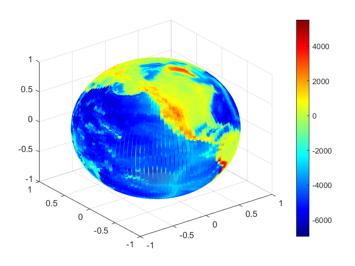
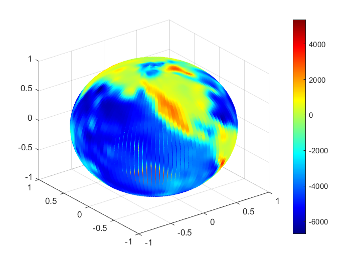
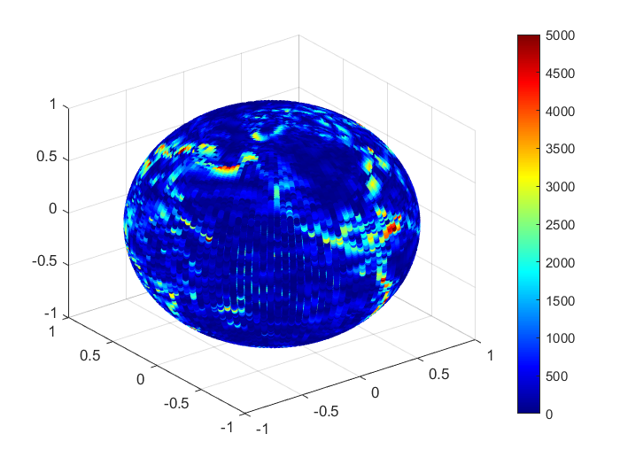
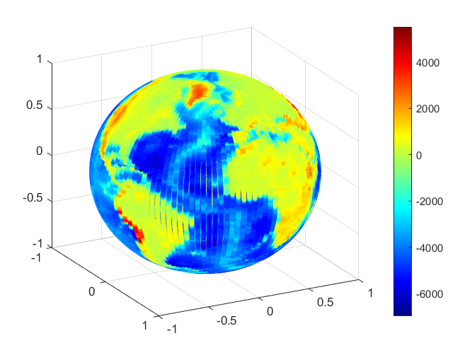
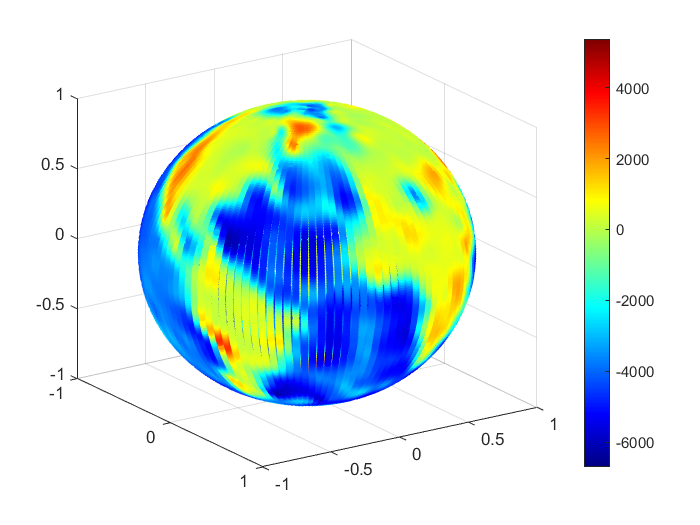
To illustrate the practical benefits of this operator, we use topographic data available from the National Geophysical Data Center, NOAA US Department of Commerce, that are available in Matlab by using the command load topo. The data is represented as an array of size . Each cell, of size (latitude and longitude), stores average altitudes (in meters) above and below the sea level [29]. The topographic map of values is shown in Figure 1. For data reconstruction based on the operator , given in (4.4), we used 1063 nodes. The approximation values and errors are displayed in Figure 2. The mean errors are about meters. Figure 3 shows the real data and the computed values from a different angle.
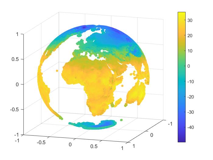
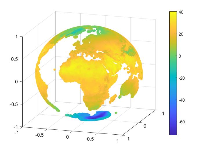
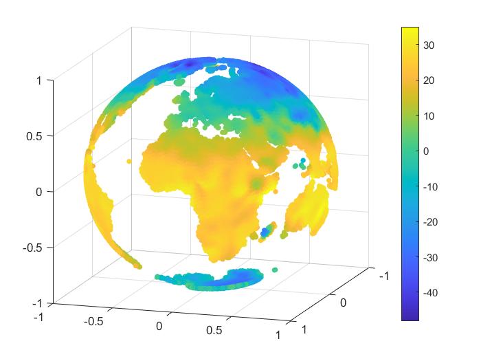
Finally, we present an application for monthly mean temperature predictions, based on a set of data downloaded from https://www.kaggle.com/datasets/shishu1421/global-temperature?select=air_temp.2010. We considered interpolation nodes and using the operator given in (4.4), we reconstructed temperature values on the Globe from January 2010 and June 2010, respectively. A map representing the real values is shown in Figure 4. The computed values are displayed in Figure 5. Finally, Figure 6 shows the approximation errors. We computed the mean approximation errors () and the root mean squared errors () to compare the results with the ones obtained in the case of the spherical Shepard operators combined with the least squares thin-plate spline () and the inverse multiquadric () functions introduced by us in [8], using the same sets of data. The results are listed in Table 7, showing that the methods are comparable.
| January | June | |||||
|---|---|---|---|---|---|---|
January 2010 and June 2010.
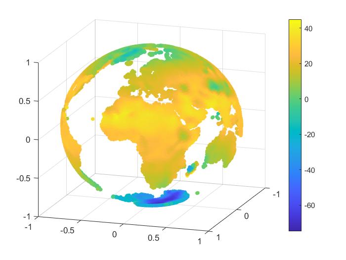
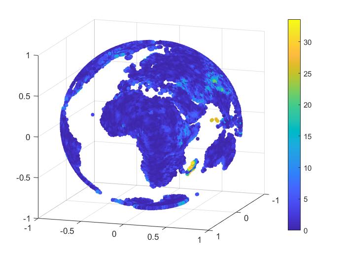
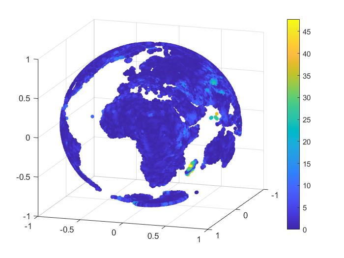
Conclusions. We have constructed the new spherical operators based on two types of Shepard basis functions and the Bernoulli operators. The last ones were considered on triangular domains. The numerical tests and the practical applications considered here for modeling some real-life phenomena demonstrated the efficiency of the proposed methods.
In our future studies, we also intend to generalize some Lidstone type operators for scattered data sets on the sphere [9].
Acknowledgments. We are grateful to the referees for the careful reading and for their valuable suggestions that improved the manuscript.
Conflict of interest statement: Not Applicable.
References
- [1] Allasia, G., Cavoretto, R., De Rossi, A.: Hermite-Birkhoff interpolation on scattered data on the sphere and other manifolds. Appl. Math. Comput. 318, 35–50 (2018)
- [2] Caira, R., Dell’Accio, F.: Shepard-Bernoulli Operators. Math. Comp. 76, 299–321 (2007).
- [3] Caira, R., Dell’Accio, F., Di Tommaso, F.: On the bivariate Shepard-Lidstone operators, Journal of Computational and Applied Mathematics, 236 (7) 1691-1707 (2012).
- [4] Cătinaş, T.: The combined Shepard-Lidstone bivariate operator. In: Trends and Applications in Constructive Approximation. International Series of Numerical Mathematics (de Bruin, M.G. et al. (eds.)), 151, pp. 77–89, Springer Group-Birkhäuser Verlag (2005)
- [5] Cătinaş, T.: The bivariate Shepard operator of Bernoulli type. Calcolo 44(4), 189–202 (2007)
- [6] Cătinaş, T., Malina, A.: Shepard operator of least squares thin-plate spline type. Stud. Univ. Babeş-Bolyai Math. 66(2), 257–265 (2021)
- [7] Cătinaş T, Malina A.: The combined Shepard operator of inverse quadratic and inverse multiquadric type. Stud. Univ. Babeş-Bolyai Math. 67, 579-–589 (2022)
- [8] Cătinaş, T., Malina, A.: Spherical interpolation of scattered data using least squares thin-plate spline and inverse multiquadric functions. Numer Algor (2024). https://doi.org/10.1007/s11075-024-01755-6
- [9] Cătinaş, T., Malina, A.: Spherical Shepard-Lidstone type operators, manuscript.
- [10] Cavoretto, R., De Rossi, A.: Fast and accurate interpolation of large scattered data sets on the sphere. J. Comput. Appl. Math. 234, 1505–1521 (2010)
- [11] Cavoretto, R., De Rossi, A.: Numerical comparison of different weights in Shepard’s interpolants on the sphere. Appl. Math. Sci. 4, 3425–3435 (2010)
- [12] Cavoretto, R., De Rossi, A.: Spherical interpolation using the partition of unity method: An efficient and flexible algorithm. Appl. Math. Lett. 25, 1251–1256 (2012)
- [13] Cavoretto, R., De Rossi, A.: Achieving accuracy and efficiency in spherical modelling of real data. Math. Methods Appl. Sci. 37, 1449–1459 (2014)
- [14] Cavoretto, R., De Rossi, A., Dell’Accio, F., Di Tommaso, F.: Fast computation of triangular Shepard interpolants. J. Comput. Appl. Math. 354, 457–470 (2019)
- [15] Cavoretto, R., De Rossi, A., Dell’Accio, F., Di Tommaso, F.: An efficient trivariate algorithm for tetrahedral Shepard interpolation. J. Sci. Comput. 82, 57 (2020)
- [16] Costabile, F.A., Dell’Accio, F.: Expansion over a rectangle of real functions in Bernoulli polynomials and applications. BIT 41, 451–-464 (2001).
- [17] Costabile, F.A., Dell’Accio, F.: Expansion over a simplex of real functions by means of Bernoulli polynomials. Numer Algorithms 28, 63–-86 (2001).
- [18] Costabile, F.A., Dell’Accio, F.: Lidstone Approximation on the Triangle, Appl. Numer. Math., 52 339-361 (2005).
- [19] Costabile, F.A., Dell’Accio, F., Gualtieri, M.I.: A new approach to Bernoulli polynomials, Rendiconti di Matematica e delle sue Applicazioni 26, 1-12 (2006).
- [20] Costabile, F.A., Dell’Accio, F., Guzzardi, L.: New bivariate polynomial expansion with boundary data on the simplex, Calcolo, 45 177-192 (2008).
- [21] Costabile, F.A., Dell’Accio, F., Di Tommaso, F., Complementary Lidstone Interpolation on Scattered Data Sets, Numerical Algorithms, 64 157-180 (2013).
- [22] Dell’Accio, F., Di Tommaso, F., Hormann, K.: On the approximation order of triangular Shepard interpolation. IMA J. Numer. Anal. 36, 359–379 (2016).
- [23] Dell’Accio, F., Di Tommaso, F.: Bivariate Shepard-Bernoulli operators. Math. Comput. Simulation 141, 65–82 (2017)
- [24] Dell’Accio, F., Di Tommaso, F., Nouisser, O., Zerroudi, B.: Increasing the approximation order of the triangular Shepard method. Appl. Numer. Math. 126, 78–91 (2018)
- [25] De Rossi, A.: Spherical interpolation of large scattered data sets using zonal basis functions. In: Mathematical Methods for Curves and Surfaces (Daehlen, M., Morken, K., Schumaker, L. (eds.)), pp. 125–134, Trømso 2004. Nashboro Press (2005)
- [26] Farwig, R.: Rate of convergence of Shepard’s global interpolation formula. Math. Comp. 46, 577–590 (1986)
- [27] Franke, R.: Scattered data interpolation: tests of some methods. Math. Comp. 38, 181–200 (1982)
- [28] Franke, R., Nielson, G.: Smooth interpolation of large sets of scattered data. Int. J. Numer. Meths. Engrg. 15, 1691–1704 (1980)
- [29] Le Gia, Q., Sloan, I., Wendland, H.: Multiscale Analysis in Sobolev Spaces on the Sphere. SIAM J. Numerical Analysis. 48, 2065-–2090 (2010)
- [30] Little, F.: Convex combination surfaces. In: Surfaces in Computer Aided Geometric Design (Barnhill, R.E., Boehm, W. (eds)), pp. 99–107, Amsterdam: North-Holland (1983).
- [31] Nielson, G., Ramaraj, R.: Interpolation over a sphere based upon a minimum norm network. Comput. Aided Geom. Design 4, 41–57 (1987).
- [32] Renka, R.J.: Interpolation of data on the surface of a sphere. ACM Trans. Math. Software 10, 417–436 (1984).
- [33] Renka, R.J., Cline, A.K.: A triangle-based interpolation method. Rocky Mountain J. Math. 14, 223–237 (1984)
- [34] Renka, R.J.: Multivariate interpolation of large sets of scattered data. ACM Trans. Math. Software 14, 139–148 (1988)
- [35] Renka, R.J.: Algorithm 772: STRIPACK, Delaunay Triangulation and Voronoi Diagram on the Surface of a Sphere. ACM Trans. Math. Software 23, 416-–434 (1997).
- [36] Saff, E.B., Kuijlaars, A.B.J.: Distributing many points on a sphere. Math. Intelligencer. 19, 5–11 (1997)
- [37] Shepard, D.: A two dimensional interpolation function for irregularly spaced data. In: Proceedings of the 1968 23rd ACM National Conference, 517–523. ACM (1968)
- [38] Wong, T.T., Luk, W.S., Heng, P.A.: Sampling with Hammersley and Halton Points. J. Graph. Tools, 2(2), 9–24 (1997)
- [39] Zerroudi, B., Tayeq, H., El Harrak, A.: Effective interpolation of scattered data on a sphere through a Shepard-like method. Math. Model. Comput., 10(4), 1174-–1186 (2023)
- [40] Zerroudi, B., Tayeq, H., El Harrak, A.: Scattered data interpolation on the 2-dimensional surface through Shepard-like technique. Math. Model. Comput., 11(1), 277–-289 (2024)
- [41] Zuppa, C.: Error estimates for moving least square approximations. Bull. Braz. Math. Soc. (N.S), 34(2), 231–249 (2003)
- [42] https://github.com/andramalina/Shepard-Bernoulli-sphere
1. Allasia, G., Cavoretto, R., De Rossi, A.: Hermite-Birkhoff interpolation on scattered data on the sphere and other manifolds. Appl. Math. Comput. 318, 35–50 (2018)
2. Caira, R., Dell’Accio, F.: Shepard-Bernoulli operators. Math. Comp. 76, 299–321 (2007)
3. Caira, R., Dell’Accio, F., Di Tommaso, F.: On the bivariate Shepard-Lidstone operators. J. Comput. Appl. Math. 236(7), 1691–1707 (2012)
4. Cătinaș, T.: The combined Shepard-Lidstone bivariate operator. In: Trends and Applications in Constructive Approximation. International Series of Numerical Mathematics (de Bruin,M.G. et al. (eds.)), 151, pp. 77–89, Springer Group-Birkhäuser Verlag (2005)
5. Cătinaș, T.: The bivariate Shepard operator of Bernoulli type. Calcolo 44(4), 189–202 (2007)
6. Cătinaș, T., Malina, A.: Shepard operator of least squares thin-plate spline type. Stud. Univ. Babeș-Bolyai Math. 66(2), 257–265 (2021)
7. Cătinaș, T., Malina, A.: The combined Shepard operator of inverse quadratic and inverse multiquadric type. Stud. Univ. Babeș-Bolyai Math. 67, 579–589 (2022)
8. Cătinaș, T., Malina, A.: Spherical interpolation of scattered data using least squares thin-plate spline and inverse multiquadric functions. Numer. Algor. (2024). https://doi.org/10.1007/s11075-024-01755-6
9. Cătinaș, T., Malina, A.: Spherical Shepard-Lidstone type operators, manuscript
10. Cavoretto, R., De Rossi, A.: Fast and accurate interpolation of large scattered data sets on the sphere. J. Comput. Appl. Math. 234, 1505–1521 (2010)
11. Cavoretto, R., De Rossi, A.: Numerical comparison of different weights in Shepard’s interpolants on the sphere. Appl. Math. Sci. 4, 3425–3435 (2010)
12. Cavoretto, R., De Rossi, A.: Spherical interpolation using the partition of unity method: an efficient and flexible algorithm. Appl. Math. Lett. 25, 1251–1256 (2012)
13. Cavoretto, R., De Rossi, A.: Achieving accuracy and efficiency in spherical modelling of real data. Math. Methods Appl. Sci. 37, 1449–1459 (2014)
14. Cavoretto, R., De Rossi, A., Dell’Accio, F., Di Tommaso, F.: Fast computation of triangular Shepard interpolants. J. Comput. Appl. Math. 354, 457–470 (2019)
15. Cavoretto, R., De Rossi, A., Dell’Accio, F., Di Tommaso, F.: An efficient trivariate algorithm for tetrahedral Shepard interpolation. J. Sci. Comput. 82, 57 (2020)
16. Costabile, F.A., Dell’Accio, F.: Expansion over a rectangle of real functions in Bernoulli polynomials and applications. BIT 41, 451–464 (2001)
17. Costabile, F.A., Dell’Accio, F.: Expansion over a simplex of real functions by means of Bernoulli polynomials. Numer. Algorithms 28, 63–86 (2001)
18. Costabile, F.A., Dell’Accio, F.: Lidstone Approximation on the Triangle. Appl. Numer. Math. 52, 339–361 (2005)
19. Costabile, F.A., Dell’Accio, F., Gualtieri, M.I.: A new approach to Bernoulli polynomials. Rendiconti di Matematica e delle sue Applicazioni 26, 1–12 (2006)
20. Costabile, F.A., Dell’Accio, F., Guzzardi, L.: New bivariate polynomial expansion with boundary data on the simplex. Calcolo 45, 177–192 (2008)
21. Costabile, F.A., Dell’Accio, F., Di Tommaso, F.: Complementary Lidstone Interpolation on Scattered Data Sets. Numer. Algorithms 64, 157–180 (2013)
22. Dell’Accio, F., Di Tommaso, F., Hormann, K.: On the approximation order of triangular Shepard interpolation. IMA J. Numer. Anal. 36, 359–379 (2016)
23. Dell’Accio, F., Di Tommaso, F.: Bivariate Shepard-Bernoulli operators. Math. Comput. Simulation 141, 65–82 (2017)