Abstract
?
Author
Ion Păvăloiu
(Tiberiu Popoviciu Institute of Numerical Analysis)
Keywords
?
Cite this paper as:
I. Păvăloiu, On the monotonicity of the sequences of approximations obtained by Steffensen’s method, Mathematica, 35(58) (1993) no. 1, pp. 71-76.
About this paper
Journal
Mathematica – Revue d’analyse numérique et de théorie de l’approximation.
Mathematica
Publisher Name
Editions de l’Academie Roumaine
DOI
Not available yet.
Print ISSN
Not available yet.
Online ISSN
Not available yet.
References
[1] Balazs, M., A bilateral approximating method for finding the real roots of real equations. Rev. Anal. Numer. Theor. Approx., 21, no. 2, 111–117, (1992).
[2] Pavaloiu, I., Sur la methode de Steffensen pour la resolution des equations operationnelles non lineaires, Revue Roumaine des Mathematiques Pures et Appliquees, XIII, 6, 149–158 (1968).
[3] Pavaloiu, I., Rezolvarea ecuatiilor prin interpolare, Ed. Dacia, Cluj-Napoca (1981).
[4] Ul’m, S., Ob obobschenie metoda Steffensen dlya reshenia nelineinyh operatornyh uravnenii, Jurnal Vicisl, mat. i. mat-fiz. 4, 6, (1964).
Paper (preprint) in HTML form
On the monotonicity of the sequences of approximations obtained by
Steffensen’s method
In a recent paper [1], M. Bálazs studied the conditions in which the sequence generated by Steffensen’s method is monotonic and converges to the solution of equation
| (1) |
where is a given function, and is an interval of the real axis. Paper [1] considers the simple case of the sequence generated by the recurrence relation
| (2) |
in which is given by and is the first order divided difference of the function
The following theorem is proved in [1]:
Theorem 1.
[1]. Let be a continuous function on and define If the following conditions:
-
(i)
The function is strictly decreasing and convex on
-
(ii)
there exists a point such that
-
(iii)
where
hold, then all elements of the sequence generated by (2) belong to in addition, the following properties hold:
-
(j)
the sequence is increasing and convergent;
-
(jj)
the sequence is decreasing and convergent;
-
(jjj)
where is the unique solution of equation (1) in
We shall show further down that the properties resulting from Theorem 1 hold for more general Steffensen-type methods, while for the method (2), if hypothesis (ii) is replaced by:
-
(ii1)
there exists for which and then hypothesis (iii) can be dropped, and the conclusions of the theorem remain valid putting
Consider an arbitrary function whose fixed points coincide with the real roots of equation (1), and reciprocally.
The following theorem holds:
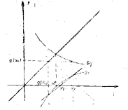
Theorem 2.
If the functions and are continuous on and if the following conditions:
-
(i2)
the function is strictly decreasing on
-
(ii2)
the function is strictly increasing and concave on
-
(iii2)
there exists such that and
-
(iv2)
the equations and are equivalent, are fulfilled then equation (1) has a unique solution and the following properties hold:
-
(j2)
the sequence is decreasing and convergent;
-
(jj2)
the sequence is increasing and convergent;
-
(jjj2)
where is the unique solution of equation (1), therefore fixed point of in the interval
Proof.
Writing we have by hypothesis; moreover:
hence the equation has unique solution in the interval i.e. has a unique fixed point in this interval. Since the fixed points of coincide with the roots of equation (1) and reciprocally, there follows that is unique solution for equation (1) within the same interval, and Now we shall show that First show that
It is easy to verify that the terms of the sequence provided by the relations
coincide with those of the sequence generated by (2). In other words the equalities
hold; for it follows that:
from which it results that
From Lagrange’s interpolating polynomial we get
and, since taking into account (2), it follows that that is, Since the function is increasing, it results that , i.e. Let us show that We have that is,
Repeating the above argument, putting , and supposing that the hypotheses of Theorem 2 are fulfilled for we obtain:
It results subsequently that the sequences and fulfil the properties (j2) and (jj2) of Theorem 2 and, in addition, are bounded.
Write and we obtain and Suppose that therefore . But since this shows that
At limit (for ), equalities (2) yield where the continuity of was also taken into account. ∎
Remark 1.
If we put in Theorem 2, since is decreasing, it follows that is increasing; since is convex, it follows that for every hence that is, is concave. From it follows i.e. In this case, Theorem 1 in which hypotheses (ii) and (iii) are replaced by (ii2) is a consequence of Theorem 2.
In what follows we shall present, without proof. other cases in which properties of monotonicity analogous to those given by Theorem 2 hold.∎
Theorem 3.
If the functions and are continuous on and if the following conditions are fulfilled:
-
(i3)
the function is strictly decreasing on
-
(ii3)
the function is strictly increasing and convex on
-
(iii3)
there exists for which and
- (iv3)
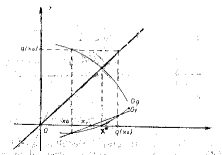
Theorem 4.
If the functions and are continuous on and if the following conditions are fulfilled:
-
(i4)
the function is strictly decreasing on
-
(ii4)
the function is strictly decreasing and convex on
-
(iii4)
there exists for which and
-
(iv4)
the equations and are equivalent, then the sequence generated by (2) is decreasing and convergent, the sequence is increasing and convergent, and
The results of this theorem are illustrated by Figure 3.
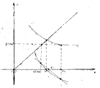
Theorem 5.
If the functions and are continuous on and if the following conditions are fulfilled:
-
(i5)
the functions is strictly decreasing on
-
(ii5)
the function is strictly decreasing and concave on
-
(iii5)
there exists such that and
-
(iv5)
the equations and are equivalent then the sequence generated by (2) is increasing and convergent, the sequence is decreasing and convergent, and
Remark 2.
The fact that the functions and from the above theorems are related only by the equivalence of equations and offers large possibilities to choose these functions (i.e. to choose when is known, and conversely).
It is clear that if keeps the same monotonicity and convexity on then we can moot the question of determining a real number such that be a decreasing function. Under certain conditions can be determined, as it results from the following example:
If is strictly increasing and strictly convex on and if is differentiable, then is also derivable, and for every Then we can put and we have for every hence is decreasing. It is clear that the equations and have the same roots. If and then it is obvious that and Theorem 3 can be applied for ∎
Numerical example.
Consider the equation:
and the function given by the relation:
Since and it follows that is decreasing on and is increasing and convex. One shows by direct calculation that and hence fulfils the hypotheses of Theorem 3. The table below lists the results of the calculations for
| 0 | -2.000000000000000000 | -1.249045772398254430 | -0.750954227601745574 |
|---|---|---|---|
| 1 | -1.414047729532868260 | -1.400933154002817630 | -0.013114575530050630 |
| 2 | -1.404227441155695550 | -1.404222310683232820 | -0.000005130472462734 |
| 3 | -1.404223602392559510 | -1.404223602391771120 | -0.000000000000788388 |
| 4 | -1.404223602391969620 | -1.404223602391969620 | -0.000000000000000000 |
The numerical results agree with the conclusions of Theorem 3; as one can see, after four iteration steps a solution approximation with 18 decimals is obtained (obviously, if truncation and rounding errors are neglected).∎
References
- [1] Balázs, M., ††margin: clickable A bilateral approximating method for finding the real roots of real equations. Rev. Anal. Numér. Théor. Approx., 21, no. 2, 111–117, (1992).
- [2] ††margin: clickable Păvăloiu, I., Sur la methode de Steffensen pour la résolution des équations operationnelles non lineaires, Revue Roumaine des Mathematiques Pures et Appliquees, XIII, 6, 149–158 (1968).
- [3] Păvăloiu, I., ††margin: clickable Rezolvarea ecuaţiilor prin interpolare, Ed. Dacia, Cluj-Napoca (1981).
- [4] Ul’m, S., Ob obobschenie metoda Steffensen dlya reshenia nelineinyh operatornyh uravnenii, Jurnal Vicisl, mat. i. mat-fiz. 4, 6, (1964).
Received 18.VI.1992
Institutul de Calcul al Academiei
Filiala Cluj
3400 Cluj-Napoca
Romania