The Shepard operator was introduced by Donald Shepard in Shepard, 1968 as an interpolation method used in scattered data approximation. It is based on a linear combination between inverse distance weights (usually Euclidean distance) and the values of an unknown function \(f\) on a set of data sites \(\mathcal{X} = \{\mathbf{x}_1,\ldots,\mathbf{x}_K\}\).
Consider \(f: X \subseteq \mathbb{R}^2 \to \mathbb{R}\) with known values \(f_i = f(x_i, y_i),\; i=1, \ldots, K,\) on a scattered data set \(\mathcal{X} = \{(x_i,y_i),\; i=1,\ldots, K\} \subset X\). The operator is defined as
$$
S_{\mu}f(x,y) = \sum_{i=1}^K A_{i, \mu}(x,y) f(x_i,y_i),
$$
with the weight functions \(A_{i, \mu}\) given by
$$
A_{i,\mu}\left( x,y\right) =\frac{\displaystyle \prod_{j=1, j \neq i}^{K}d_{j}^{\mu}\left( x,y\right)}{\displaystyle \sum_{k=1}^{K}\prod_{j=1, j\neq k}^{K}d_{j}^{\mu}\left( x,y\right) },
$$
with \(\mu>0\) and \(d_{i}\left(x,y\right)\) the Euclidean distances between \(\left( x,y\right) \in X\) and the scattered points \(\left( x_{i},y_{i}\right) \in \mathcal{X} ,\;i=1,…,K\).
We have the following properties:
- \( A_{i, \mu} (x_j,y_j) = \delta_{ij} \), for each \( i,j = 1,\ldots, K \);
- \( \sum_{i=1}^{K} A_{i, \mu}(x,y) = 1 \);
- \( S_{\mu}f(x_i,y_i) = f(x_i,y_i),\; i=1,\ldots,K \);
- the degree of exactness of \( S_\mu f \) is 0;
- \( \min_{i=1,\ldots,K} f(x_i,y_i) \leq S_{\mu}f(x,y) \leq \max_{i=1,\ldots,K} f(x_i,y_i) \).
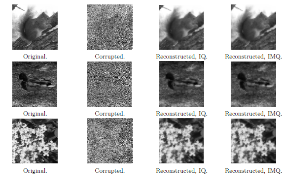
To improve the operator, several methods have been proposed. For instance, to increase the degree of exactness and for better approximation results, the function values \(f_i\) have been replaced by the values of other interpolation operators: Lagrange, Hermite, Birkhoff, Taylor, Bernoulli (Cătinaș, 2007, Dell’Accio & Di Tommaso, 2017), Lidstone (Cătinaș, 2005, Caira, Dell’Accio & Di Tommaso, 2012, Costabile, Dell’Accio & Di Tommaso, 2013), Abel-Goncharoff.
To improve the accuracy of this global method, Franke and Nielson Franke & Nielson, 1980 proposed a local approach, further developed in Franke, 1982 and Renka, 1988, which assures that only the nodes around the approximation point have a greater influence on the approximation result. Known as the modified Shepard operator, it is defined as
$$
S_{W}f(x,y) = \sum_{i=1}^{K} \overline{w}_{i,\mu}(x,y) f(x_i,y_i),
$$
with
$$
\overline{w}_{i,\mu}(x,y) = \frac{w_{i,\mu}(x,y)}{\displaystyle \sum_{j=1}^{K} w_{j,\mu}(x,y)},
$$
for
$$
w_{i,\mu}(x,y) = \left[ \frac{\left(R_w-d_i(x,y)\right)_+}{R_w d_i(x,y)} \right]^{\mu},\; \mu >0,
$$
considering \(d_i(x,y)\) as the Euclidean distance between the \(i\)th node and the point \((x,y)\), and \(R_w\) a radius of influence that varies with \(i\), chosen such that it is large enough to include \(N_w\) nodes, \(N_w\) fixed. Similar properties as for \(A_{i, \mu}\) can be proved for the weights \(w_{i,\mu}\). Similar results as in the bivariate case have been studied in the univariate case as well.
Recently, authors have started to study the interpolation problem on the sphere, due to its large number of practical applications. Consider a set of distinct nodes \(\mathcal{X}=\{\mathbf{x}_{i} = (x_i, y_i, z_i), i=1,…,K\}\) on the unit sphere \(S^2\) together with the function values \(f_{i}=f(\mathbf{x}_i),\;i=1,…,K\), with \(f: S^2 \to \mathbb{R}\). For \(\mathbf{x}=(x,y,z) \in S^2\) the modified spherical Shepard operator is given by
$$
S(\mathbf{x}) = \sum_{j=1}^{K} \overline{w}_{j}(\mathbf{x})f_{j},
$$
with
$$
\overline{w}_{j}(\mathbf{x}) = \frac{w_{j}(\mathbf{x})}{\displaystyle \sum_{k=1}^{K} w_{k}(\mathbf{x})}.
$$
The weights \(w_j\) are given as
$$
w_{j}\left(\mathbf{x} \right) =\left[ \frac{(R^{w}_j-g(\mathbf{x}, \mathbf{x}_j))_{+}}{R^{w}_jg(\mathbf{x}, \mathbf{x}_j)} \right] ^{\mu},
$$
considering \(R_{j}^{w}\) a radius of influence about the node \(j\) and \(g\) the geodesic distance between \(\mathbf{x}\) and \(\mathbf{x}_j\), i.e., \(g(\mathbf{x}, \mathbf{x}_j) = \arccos{(\mathbf{x} \cdot \mathbf{x}_j)}\).
The weights \(\overline{w}_j\) have the following properties:
- \( \overline{w}_j(\mathbf{x}_i) = \delta_{ij} \);
- \( \sum_{j=1}^{K}\overline{w}_j(\mathbf{x}) = 1 \).
As in the previous case, for better approximation results, the function values \(f_j\) have been replaced by the values of other operators such as Hermite-Birkhoff (Allasia, Cavoretto & De Rossi, 2017) or Bernoulli (Cătinaș & Malina, 2025) and by the values of some spherical radial basis functions (Cătinaș & Malina, 2024, De Rossi, 2005, Cavoretto & De Rossi, 2010, Cavoretto & De Rossi, 2010).