We survey the convergence orders of sequences and show the orders of the basic iterative sequences for solving nonlinear equations in \({\mathbb R}\): the Newton method, the secant method, and the successive approximations).
Abstract
The high speed of \(x_{k}\rightarrow x^\ast\in{\mathbb R}\) is usually measured using the C-, Q- or R-orders:
\begin{equation}\tag{$C$}
\lim \frac {|x^\ast – x_{k+1}|}{|x^\ast – x_k|^{p_0}}\in(0,+\infty),
\end{equation}
\begin{equation}\tag{$Q$}
\lim \frac {\ln |x^\ast – x_{k+1}|}{\ln |x^\ast – x_k|} =q_0,
\qquad \mbox{resp.}
\end{equation}
\begin{equation}\tag{$R$}
\lim \big\vert\ln |x^\ast – x_k| \big \vert ^\frac1k =r_0.
\end{equation}
By connecting them to the natural, term-by-term comparison of the errors of two sequences, we find that the C-orders — including (sub)linear — are in agreement. Weird relations may appear though for the Q-orders: we expect
\[
|x^\ast – x_k|=\mathcal{O}(|x^\ast – y_k|^\alpha), \qquad\forall\alpha>1,
\]
to attract “\(\geq\)” for the Q-orders of \(\{x_{k}\}\) vs. \(\{y_{k}\}\); the contrary is shown by an example providing no vs. infinite Q-orders. The R-orders seem even worse: an \(\{x_{k}\}\) with infinite R-order may have unbounded nonmonotone errors: \(\limsup \)\(|x^\ast – x_{k+1}|/|x^\ast – x_k|= +\infty\).
Such aspects motivate the study of equivalent definitions, computational variants, etc.
The orders are also the perspective from which we analyze the three basic iterative methods for nonlinear equations. The Newton method, widely known for its quadratic convergence, may in fact attain any C-order from \([1,+\infty]\) (including sublinear); we briefly recall such convergence results, along with connected aspects (historical notes, known asymptotic constants, floating point arithmetic issues, radius of attraction balls, etc.) and provide examples.
This approach leads to similar results for the successive approximations, while the secant method exhibits different behavior: it may not have high C-, but just Q-orders.
Authors
Keywords
(computational) convergence orders, iterative methods, Newton method, secant method, successive approximations, asymptotic rates.
here you may find an annotated version, with some typos pointed out: https://ictp.acad.ro/wp-content/uploads/2023/12/Catinas-2021-SIREV-How-many-steps-still-left-to-x-annotated.pdf
also freely available at the publisher (without pointed typos): http://doi.org/10.1137/19M1244858
Paper coordinates:
E. Catinas, How many steps still left to x*?, SIAM Rev., 63 (2021) no. 3, pp. 585–624, doi: 10.1137/19M1244858
About this paper
Print ISSN
0036-1445
Online ISSN
1095-7200
Github
Some small codes in LaTeX and Julia have been posted on Github in order to illustrate some aspects.
We will post soon in Python too.
The link is: https://github.com/ecatinas/conv-ord
Corrigendum
(introduced on February 10, 2023, modified on February 25, 2023, on August 27, 2023)
Corrigendum:
- for the sequences with \(\bar{Q}_1=\infty\) we have proposed the terminology “sequences with unbounded nonmonotone errors” (see Remark 2.12.c). This is also termed in the beginning of Section 2.2 as “sequences with no Q-order” – which is not proper, as we have subsequently found sequences with \(\bar{Q}_1=\infty\) and with Q-order \(1\), see [Cătinaş, 2023];
- in Remark 2.50.b, “the strict superlinear” should be removed. Indeed, this is not a C-order, but a Q-order, as is defined with the aid of \(\bar{Q}_p\). On the other hand, the strict superlinear order is not always faster than the C-order \(p>1\), see [Cătinaş, 2023].
Typos:
- in the abstract, condition \(|x^\ast – x_{k+1}|/|x^\ast – x_{k}| \rightarrow \infty\) (i.e., \(Q_1=\infty\)), for the sequence with unbounded nonmonotone error, should read instead \(\limsup |x^\ast – x_{k+1}|/|x^\ast – x_{k}| = \infty\) (i.e., \(\bar{Q}_1=\infty\)); obviously, condition \(Q_1=\infty\) cannot be fulfilled by a convergent sequence. The matter is correctly dealt with inside the paper (see Remark 2.12.c).
Notes
Working with the SIAM staff was an amazing experience. I would like to thank to Louis Primus for his solicitude and professionalism.
Version: October 30, 2021.
Some references I have missed:
(these were included in the initial submission, but missing in the final version, as not cited in text, and we switched to BibTeX)
- M. Grau-Sánchez, M. Noguera, A. Grau, J.R. Herrero, On new computational local orders of convergence, Appl. Math. Lett. 25 (2012) 2023–2030, doi: 10.1016/j.aml.2012.04.012
- I. Pavaloiu, Approximation of the roots of equations by Aitken-Steffensen-type monotonic sequences, Calcolo 32 (1–2) (1995) 69–82, doi: 10.1007/BF02576543.
- I. Pavaloiu, On the convergence of one step and multistep iterative methods, Unpublished manuscript, https://ictp.acad.ro/convergence-one-step-multistep-iterative-methods/.
known to me, but still missing (nobody is perfect):
- N. Bicanic and K. H. Johnson, Who was ’-Raphson’?, Intl. J. Numerical Methods Engrg., 14 (1979), pp. 148–152, https://doi.org/10.1002/nme.1620140112.
- A. Melman, Geometry and convergence of Euler’s and Halley’s methods, SIAM Rev., 39 (1997), pp. 728–735, https://doi.org/10.1137/S0036144595301140.
- S. Nash, Who was -Raphson? (an answer), NA Digest, 92 (1992).
found after sending the revised version:
- J. H. Wilkinson, The evaluation of the zeros of ill-conditioned polynomials. part ii, Numer. Math., 1 (1959), pp. 167–180, doi: 10.1007/BF01386382
- D. F. Bailey and J. M. Borwein, Ancient indian square roots: an exercise in forensic paleo mathematics, Amer. Math. Monthly, 119 (2012), pp. 646–657, doi 10.4169/amer.math.monthly.119.08.646.
- E. Halley, Methodus nova accurata & facilis inveniendi radices aeqnationum quarumcumque generaliter, sine praviae reductione, Phil. Trans. R. Soc., 18 (1694), pp. 136–148, https://doi.org/10.1098/rstl.1694.0029.
- A. Ralston and P. Rabinowitz, A First Course in Numerical Analysis, 2nd ed., 1978.
- M. A. Nordgaard, The origin and development of our present method of extracting the square and cube roots of numbers, The Mathematics Teacher, 17 (1924), pp. 223–238, https://doi.org/https://www.jstor.org/stable/27950616.
…
and others (to be completed)
Paper (preprint) in HTML form
How Many Steps Still Left to *?††thanks: Received by the editors February 14, 2019; accepted for publication (in revised form) September 17, 2020; published electronically August 5, 2021.
Abstract. The high speed of is usually measured using the -, -, or -orders:
By connecting them to the natural, term-by-term comparison of the errors of two sequences, we find that
the -orders—including (sub)linear—are in agreement.
Weird relations may appear though for the -orders:
we expect to imply “” for the -orders of vs. ; the contrary is shown by an example providing no vs. infinite -orders.
The -orders appear to be even worse:
an with infinite -order may have unbounded nonmonotone errors:
.
Such aspects motivate the study of equivalent definitions, computational variants, and so on.
These orders are also the perspective from which we analyze the three basic iterative methods for nonlinear equations in .
The Newton method, widely known for its quadratic convergence, may in fact attain any -order from (including sublinear);
we briefly recall such convergence results, along with connected aspects (such as historical notes, known asymptotic constants, floating point arithmetic issues, and radius of attraction balls), and provide examples.
This approach leads to similar results for the successive approximations method, while
the secant method exhibits different behavior: it may not have high -orders, but only -orders.
Keywords. (computational) convergence orders, iterative methods, Newton method, secant method, successive approximations, asymptotic rates
AMS subject classifications. 65-02, 65-03, 41A25, 40-02, 97-02, 97N40, 65H05
DOI. 10.1137/19M1244858
1 Introduction
The analysis of the convergence speed of sequences is an important task, since in numerical applications the aim is to use iterative methods with fast convergence, which provide good approximations in few steps.
The ideal setting for studying a given sequence is that of error-based analysis, where the finite limit is assumed to be known and we analyze the absolute values of the errors, . The errors allow the comparison of the speeds of two sequences in the most natural way, even if their limits are distinct (though here we write both as ). Let us first define notation, for later reference.
Notation.
Given , denote their errors by , resp., , etc.
Comparison 1.1.
converges faster (not slower) than if
| () |
(or, in brief, is eq. faster than ) and strictly faster if
| () |
Furthermore, increasingly faster convergence holds if
- for some we have
- the constant above is not fixed, but tends to zero (see, e.g., [9, p. 2], [53]),
| () |
- given , we have
| () |
Let us first illustrate the convergence speed in an intuitive fashion, using some graphs.
Example 1.2.
Consider the following two groups of sequences :
-
(a)
, , ;
-
(b)
, , , .
Handling the first terms of these sequences raises no difficulties, as all the common programming languages represent them as in standard double precision arithmetic (called binary64 by the IEEE 754-2008 standard); see 1.4 below.
The plotting of in fig. 1(a) does not help in analyzing the behavior of the errors, as for we cannot see much, even if the graph is scaled.333The implicit fitting of the figures in the window usually results in different units for the two axes (scaled graph). In fig. 1(a) we would see even less if the graph were unscaled. All we can say is that has the slowest convergence, followed by , and also that the first terms of are smaller than those of .
In order to compare the last terms we must use the semilog coordinates in fig. 1(b) (see [43, p. 211]); for , they are , belonging to the line , . As the graph is twice scaled,444The first scaling is by the use of an unequal number of units ( on axis vs. on axis ), and the second one results from the fact that the final figure is a rectangle instead of a square. it actually shows another line, .
Figure 1(b) shows that, in reality, is eq. faster than (). We will see later that the convergence is sublinear in group (a) and linear in group (b).
Exercise 1.4.
(a) The smallest positive binary64 number, which we denote by realmin( binary64 ), is . Analyzing its binary representation, express its value as a power of (see [69, p. 14], [28], or [45]).
(b) For each sequence from (a) and (b) in the example above, compute the largest such that .
(c) Give a formula for the largest index for which all the elements of all the sequences from (a) and (b) in the example above are nonzero.
Next we analyze some increasingly faster classes of sequences.
Example 1.5.
Consider
-
(c)
, , ;
-
(d)
, , , ;
-
(e)
;
-
(f)
, .
In fig. 2 we plot , , and . Their graphs are on a line (the fastest from fig. 1(b)), on a parabola , and, resp., in between.
The computation with what appears at first sight to be a “reasonable” number of terms (say, ) becomes increasingly challenging as we successively consider from (c)–(f).
We leave as an exercise the calculation/computation of the largest index for each in (c)–(f) such that is a nonzero binary64 number; we note though that all and are zero for , respectively, , and so binary64 numbers are not enough here.
There are plenty of choices for increased precision: the well-known MATLAB [58] (but with the Advanpix toolbox [1] providing arbitrary precision), the recent, freely available Julia [5], and many others (not to mention the programming languages for symbolic computation). All the graphs from this paper were obtained using the tikz/pgf package [92] for LaTeX.555The initial TeX system was created by D. E. Knuth [54]. The figures are easy to customize and the instructions to generate them have a simple form, briefly,
\addplot [domain=1:20, samples=20] {1/sqrt(x)};
Equally important, we will see that the tikz/pgf library allows the use of higher precision than binary64 (more precisely, smaller/larger numbers by increased representation of the exponent, e.g., realmin around ). The LaTeX sources for the figures are posted on https://github.com/ecatinas/conv-ord.
The sequence groups (c)–(f) are presented in fig. 3; belongs to a cubic parabola, and to an exponential. The parabola of appears flat, which shows how much faster the other sequences converge. The descent of the three terms of is the steepest.
As will be seen later, the sequence groups (c)–(f) have increasing order: strict superlinear, quadratic, cubic, and infinite, respectively.
Exercise 1.6.
Show that is eq. , faster than .
Obviously, when comparing two sequences by eq. , the faster one must have its graph below the other one () (cf. Polak [75, p. 47]). While the more concave the graph the better (cf. Kelley [50, Ex. 5.7.15]), fast convergence does not in fact necessarily require smooth graphs (see Jay [47]).
Exercise 1.7.
Consider, for instance, the merging of certain sequences.
Example 1.8.
Let
, , , , , written in eq. order of decreasing speed, are plotted in Figure 4(a). The usual ranking by convergence orders is instead , , , , (-orders , , , -order , no order). Though has the second fastest convergence, the orders actually rank it as the slowest. does not have - or -order (but just exact -order ), so is usually ranked below .
, , , from fig. 4(b) have ranking , , , (-orders , , , -order ). Though nonmonotone, has exact -order and is (at least) eq. faster than the -quadratic .
Quiz 1.9.
Given , with errors shown in fig. 5, which one is faster?
The study of errors using 1.1 seems666Of course, one cannot always compare all sequences by eq. : consider and , for example. perfect in theory, but has a notable disadvantage: it requires two sequences. The alternative is to use a “scale” for measuring any single sequence—the convergence orders. The (classical) -orders, though they demand some strong conditions, appear in the convergence of the most often encountered iterative methods for nonlinear equations.777A notable exception: the higher orders of the secant method are - but not necessarily -orders.
Still, some problems appear, for example, when one wants to check the usual predictions such as “in quadratic convergence, the error is squared at each step.” Indeed, as a sequence is an infinite set, its order refers to the asymptotic range (all sufficiently large indices), where statements such as
“if is suff. small, s.t. [some property] holds ”
come to life. Clearly, the first terms (, or perhaps ) are not necessarily connected to the order: a finite number of terms does not contribute to the order of an abstract sequence, while, most painful, the high order of an iterative method may not be reflected in its first steps if the initial approximation is not good enough. Therefore, such predictions, instead of being applicable to the very first term, are usually applied only starting from the first terms from the asymptotic range.
When the stringent conditions of -orders are not fulfilled, the -orders are considered instead, but unfortunately they can be in disagreement with the term-by-term comparison of the errors of two sequences; indeed, we show that convergence even with no - (or )-order may in fact hide a fast overall speed, only some of the consecutive errors do not decrease fast enough. The -orders are instead known for their limited usefulness, requiring the weakest conditions and allowing nonmonotone errors.
Consider now a further problem: given some iterations for which the calculation of the order turns out to be difficult or even impossible, can the computer be used to approximate it? A positive answer is given by the computational convergence orders.
Despite the fact that convergence orders have a long history, it is only recently that some final connections were made and a comprehensive picture was formed of the -, -, and -orders, together with their computational variants [20].
The understanding of these notions is important from both the theoretical and the practical viewpoints, the comments of Tapia, Dennis, and Schäfermeyer [93] being most relevant:
The distinction between - and -convergence is quite meaningful and useful and is essentially sacred to workers in the area of computational optimization. However, for reasons not well understood, computational scientists who are not computational optimizers seem to be at best only tangentially aware of the distinction.
We devote section 2 to error-based analysis of the problem of measuring and comparing convergence speeds of abstract real sequences, using either the convergence orders we review, or the term-by-term comparison of errors.
In section 3 we deal with the computational versions of the convergence orders (based either on the corrections888Each can be seen as being obtained from by adding the correction. or on the nonlinear residuals ) and show that in they are equivalent to the error-based ones.
In section 4 we deal with three main iterative methods (Newton, secant, and successive approximations), presenting results on their attainable convergence orders, as well as other connected aspects (asymptotic constants, estimation of the attraction balls, floating point arithmetic issues, brief history, etc.).
2 -, -, and -Orders vs. Asymptotic Rates
Even though the roots of iterative methods trace back to the Babylonians and Egyptians (ca. 1800 B.C.) [3], the first comment on convergence orders seems to have been made by Newton (ca. 1669) on the doubling of digits in quadratic convergence (quoted by Ypma in [101]): “But if I desire to continue working merely to twice as many figures, less one” and then in 1675: “That is, the same Division, by wch you could finde the 6th decimal figure, if prosecuted, will give you all to the 11th decimal figure.”
In the Journal Book of the Royal Society, it is recorded “17 December 1690: Mr Ralphson’s Book was this day produced by E Halley, wherein he gives a Notable Improvemt of ye method […], which doubles the known figures of the Root known by each Operation….”
Halley noticed the tripling of digits in the method he introduced.
In his Tracts, Hutton showed that one of his schemes is of third order [3]. In 1818, Fourier [38] also noted that the iterates double the exact figures at each Newton step.
In 1870, Schröder [87] implicitly defined the high -orders for some iterative methods by considering conditions on the nonlinear mapping.
Three types of convergence orders are used at present: the classical -order (notation adopted from [4]), the -order (which contains the -order as a particular case), and the -order. Outstanding contributions to their study were successively made by Ortega and Rheinboldt (1970) in their fundamental book [67], Potra and Pták (1984) [79], Potra (1989) [76], and finally by Beyer, Ebanks, and Qualls (1990), in the less known but essential paper [4]. In [20] we connected and completed these results (in ).
We analyze here only the high orders, noting that the various equivalent definitions of the -orders lead to intricate implications for linear convergence [4].
2.1 -Order
The definition of - and -orders is obtained by considering for the quotient convergence factors [67, sect. 9.1]
It is assumed that . If, though, in an iterative method, then (hopefully) we get , (this holds for the three methods in section 4).
Let us briefly list the four slowest types of -order:
-
•
no -order, when (e.g., , odd; , even);
-
•
-sublinear, if (e.g., );
-
•
-linear, if (e.g., );
-
•
-superlinear (defined later, usually called (strict) -superlinear);
notice that cannot hold, and that , with no -order, in fact are fast.
Remark 2.1.
(a) (see [65, p. 620]) -linear order implies strict monotone errors:
| (1) |
(b) -sublinear monotone errors (e.g., , even, , odd, ).
(c) , both nonmonotone, have no -order.
Exercise 2.2.
If has -sublinear and -linear order, show that is eq. faster than .
The following definition of high orders is well known; is implicitly assumed throughout this paper even if not explicitly mentioned.
Definition 2.3.
has -order if
| () |
Remark 2.4.
It is important to stress that above cannot be zero or infinite; these two cases will arise when analyzing the -orders.
By denoting (see [67, sect. 9.1], [88, p. 83])
| (2) |
condition eq. is equivalent either to relation
| () |
or to requiring that such that
| () |
Example 2.6.
(a) for some , , is the standard example for -order (). The usual instances are the -quadratic , (, resp., , ), the -cubic (, ), etc.
(b) ( given, ) also has -quadratic convergence.
(c) The -quadratic is nonmonotone, but with monotone .
(d) , , does not have -order : , .
Remark 2.8 (see, e.g., [4]).
If it exists, the -order of is unique. Indeed, if raising the power of the denominator in , the quotient tends to infinity, since . Similarly, if lowering the power, it tends to zero.
Example 2.9.
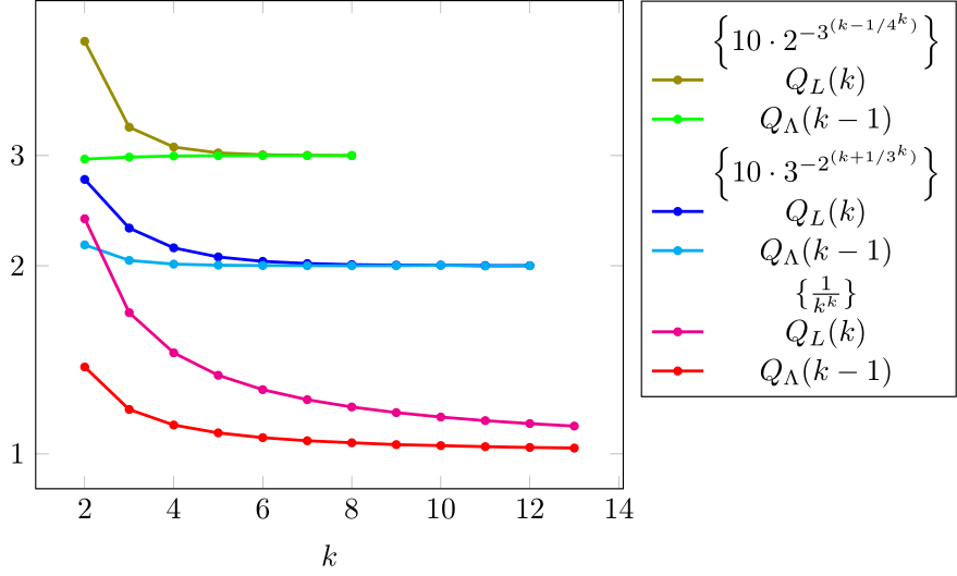
Let , , and (); in fig. 6 we plot , , and for each of them.
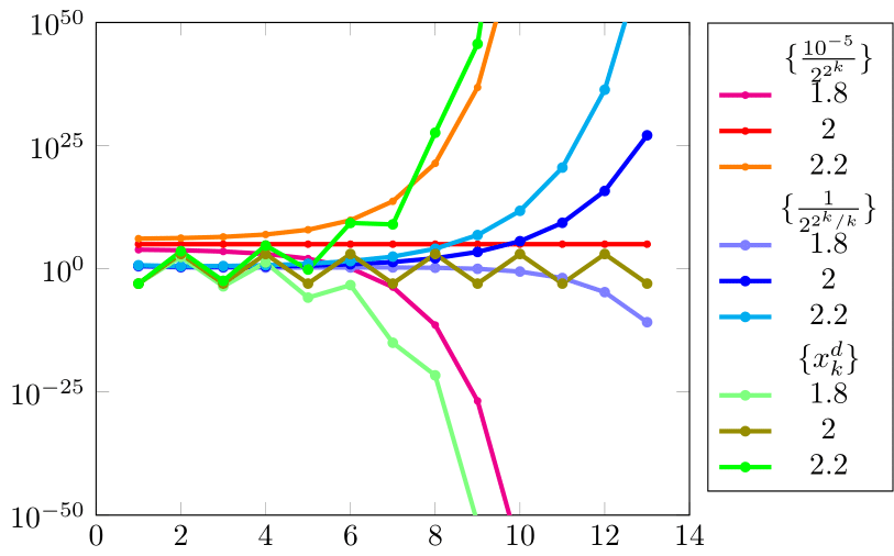
The limiting values of , from eq. 2 may be regarded as “functions” of . Their graphical illustration leads to the so-called -convergence profile of [4] (or -profile here, for short).
For all -orders , it holds that , and is a “function” given by , , and , .
In fig. 7 we plot the -profile of .
Exercise 2.10 ([4]).
Show that cannot have -order .
Exercise 2.11.
(a) Show that if has -order , then so has and
| (3) |
regardless of [20, Rem. 3.9]. Does the converse hold? (Hint: take .)
(b) [20, Rem. 3.9] Find a similar statement for .
(c) (Kelley [50, Ex. 5.7.15]) If has -order , show that is concave, i.e., is decreasing.
Not only convergence with any high order exists, but even the infinite -order, defined either by (take, e.g., [67, E 9.1-3(g)] or or by convention, when the convergence is in a finite number of steps.
“The higher the order, the better” is a well-known cliché, which we will express in section 2.5 in terms of the big Ohs.
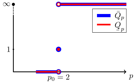
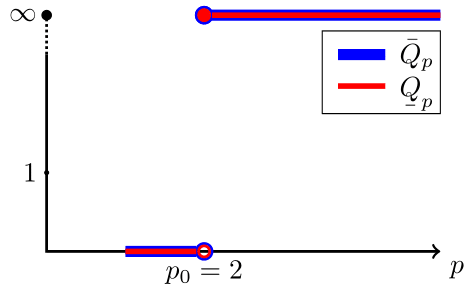
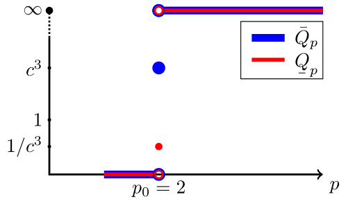
2.2 -Order
We propose the following definitions of -order convergence:
-
•
with unbounded nonmonotone errors if (e.g., );
-
•
-sublinear if (e.g., , odd, , even);
-
•
exact -sublinear if ;
-
•
at least -linear if ;
-
•
-linear if ;
-
•
exact -linear if .
Remark 2.12.
(a) Obviously, when , then and .
(b) always exist, while may not (i.e., when ).
(c) monotone, while nonmonotone errors; means unbounded nonmonotone errors. Unlike , alone does not necessarily imply slow speed (e.g., with unbounded nonmonotone errors).
The convergence may be fast when , even if (e.g., ), but is no longer fast when .
Strict -superlinear is an intermediate order between linear and .
Definition 2.13 ([67, p. 285]).
has -superlinear order999Or at least -superlinear, or even superlinear, as -superlinear is seldom encountered. if :
Strict -superlinear order holds when, moreover, .
Remark 2.14 (cf. [75, (37b)]).
-superlinear order holds if and such that and ( may be taken to be ).
Example 2.15 (strict -superlinear).
Exercise 2.16.
has -superlinear order, but not strict -superlinear order.
The following formulation has been commonly used for half a century, since the 1970 book of Ortega and Rheinboldt: “ converges with -order at least ” [67], [79], [76], [85]. Here we deal, as in [4] and [20], with a more restrictive notion, with the classic notion corresponding to the lower -order from definition 2.30.
Definition 2.17 (see [20]; cf. [76], [4]).
has -order if any of the following equivalent conditions hold:
| () | ||||
| () | ||||
| () |
or such that
| () |
Remark 2.18.
(a) If the -order exists, it is unique (recall remark 2.8).
(b) If has -order , then the right-hand side inequalities in eq. imply that the errors are strictly monotone ; see remarks 2.5 and 2.1.
In [20] we proved the equivalence of the four conditions above for , connecting and completing the independent, fundamental results of Potra [76] and Beyer, Ebanks, and Qualls [4]. This proof does not simplify for , but a natural connection between these conditions is found, e.g., by taking logarithms in eq. to obtain eq. .101010 in eq. roughly means that the number of figures is multiplied by at each step (); see, e.g., [48] and [79, p. 91]. Also, eq. and eq. can be connected by 2.11 and as follows.
Exercise 2.19.
Remark 2.20.
(a) One can always set in eq. (this is actually used in the definitions of Potra from [76]), by a proper choice of smaller and larger .
(b) In [20] we have denoted by a condition which is trivially equivalent to eq. . Here we use instead of from [20] (“” stood for “inequality” in that paper).
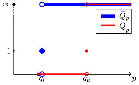
(c) eq. implies that the -profile of has a single jump at , but that the limit is not required to exist, so
| (4) |
and so six cases result for the possible values of and (, finite , ).
(d) Relations or might seem rather abstract, but they do actually occur (even simultaneously, as we shall see for the higher orders of the secant method; see also [99, p. 252 and Chap. 7], where , for a problem in ).
(e) -order implies , but the converse is not true.
fig. 8 shows the -profiles of and ().
Superlinearity may also be defined in conjunction with higher -orders, but this is tricky.
Definition 2.21 (see [47], [20]).
The -order is called
-
•
-superorder if ;
-
•
-suborder if .111111In [20] this was defined by , which we believe is not strong enough.
The -order with is -superquadratic (analogously, -supercubic, etc.).
Exercise 2.22.
(a) The -superquadratic , the - (and -)quadratic , and the -subquadratic are in eq. decreasing order of speed. Study the -order of ( is erroneous in [20]).
Example 2.23.
Let (-cubic), (-quadratic), and (-superlinear); in fig. 9 we see that tend to and , respectively.
Remark 2.24.
Plotting/comparing and avoids conclusions based on using information ahead of that from (i.e., vs. ).
The calculation of the order may be made easier by using logarithms.
Exercise 2.25.
Let .
(a) If, for some given and , one has
| (5) |
show that has -order
Thus, (the golden ratio), , , etc. Inequality eq. 5 appears in the analysis of the secant method (see theorems 4.18 and 4.22), and it does not necessarily attract - or even exact -orders, even if .
Definition 2.26 (see, e.g., [8]).
has exact -order if , s.t.
| () |
This case can be characterized in terms of the asymptotic constants .
Proposition 2.27.
has exact -order iff are finite and nonzero,
| () |
in which case the constants in eq. are bounded by
and these bounds are attained in some special restrictive circumstances.
Remark 2.29.
The classical -order of Ortega and Rheinboldt is the below.
When has -order , the lower and upper orders coincide, ; otherwise, [4]; we will also see this in theorem 2.48 (relation eq. 13).
Next we analyze from example 1.8, which has no -order, despite it being eq. faster than . We keep in mind that the -order does not measure the overall speed, but just compares the consecutive errors.
Example 2.31 ([20]).
Let with the -profile in fig. 10(a).
does not have a -order, as but still it has (exact) -order (see definitions 2.35 and 2.38). We note the usual statement in this case that “ converges with -order at least and with -order at least ,” that no longer holds in the setting of this paper.
Exercise 2.32.
Show that has and determine (here we find , and the -profile can be extended, as in [4], for ).
Determine the -profiles of and .
The inequalities implied by the lower/upper -orders are as follows.
Remark 2.33.
If , then , with , , s.t. [80]
| (7) |
(and relation eq. 6 says that is the largest value satisfying the above inequalities).
When , then such that
| (8) |
One can say that the lower -order is small when the maximum error reduction w.r.t. the previous step is small (i.e., small exponent for ). Analogously, the upper order is large when the minimum error reduction per step is small.
The role of will be seen in example 2.46.
2.3 -Order
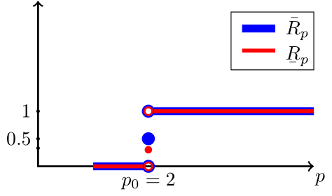
The root factors consider some averaged quantities instead of relating the consecutive terms to one another; they are defined for by
The -orders are alternatively defined by requiring the errors to be bounded by sequences converging to zero with corresponding -orders [32, p. 21], [51, Def. 2.1.3], [43, p. 218]:
Remark 2.34.
(a) At least -linear at least -linear [67, E 9.3-5], [75, Thm.1.2.41], [77], [100], [43, p. 213] (using, e.g., eq. 14); the converse is false (see above or [100]).
(b) -superlinear -superlinear, with the converse again being false (see, e.g., the above example).
Remark 2.36.
(a) If the -order exists, it is unique (see also [67, 9.2.3, p. 289]).
(b) We can always set in eq. , by choosing smaller and larger suitably (cf. [76], where was used in definitions).
(c) We prefer here the notation instead of from [20].
An example of an -profile is shown in fig. 10(b) for , with (exact) -order .
The following notion is defined similarly to the exact -order.
Definition 2.38 ([76]).
has exact -order if , s.t.
| () |
Example 2.39.
, have exact -orders : , , and , , respectively.
Exercise 2.40.
The -sub-/superquadratic , have , but not exact -order . The -sub-/superquadratic , have , respectively, , i.e., they are -sub-/superquadratic, again without having exact -order .
Remark 2.41.
Perhaps a proper definition of -superorder would be -order with , while -suborder would be -order with , .
We characterize the exact -order in the following result.
Proposition 2.42.
The exact -order of is equivalently defined by
| () |
which implies the following bounds for from eq. :
these bounds are attained in some special restrictive circumstances.
Remark 2.43.
As the -orders require weaker conditions than the -orders, they may allow nonmonotone errors. This aspect is perhaps not widely known; we have found it pointed out in [65, p. 620, and in the 1st ed.], [51, p. 14], [25, p. 51], and [47].
Clearly, iterative methods with nonmonotone errors are usually not desired.
We can easily find conditions for monotone errors in the case of exact -order .
Theorem 2.44 (monotone errors in exact -orders).
If obeys eq. and
then it has strict monotone errors ().
The lower and upper -orders, , respectively, , and further notations from [20] are
Remark 2.45.
We now consider some sequences similar to those in example 1.8.
Example 2.46.
(a) Let and take (Jay [47]).
Then converges eq. faster than and though has neither -order, nor -order, nor -order (, ), has -order .
(b) Extending the above behavior, has no -, -, or -order, but it converges eq. faster than .
(c) is eq. faster than ; has no - or -order (but has infinite -order), while has infinite -order.
Remark 2.47.
Clearly, statements such as those in the above example can appear only for sequences with , as this condition allows large upper orders . When , the corresponding sequence cannot converge quickly.
2.4 Relations between the -, -, and -Orders of a Sequence
-order of implies -order and in turn -order (see 2.22 and 2.31 for converses). We state this below and, as in [4], we use curly braces for equivalent orders.
Theorem 2.48 (see [20]; cf. [76], [4]).
Moreover, the following relation holds for the lower and upper orders:
| (13) |
Relation eq. 13 is obtained from the well-known inequalities for positive numbers,
| (14) |
Any inequality from eq. 13 may be strict. Now we see (e.g., in examples 2.31 and 2.49) that the inner inequality may be an equality (i.e., obtain -order), while one of the outer inequalities may be strict (i.e., no -order).
An with exact -order arbitrarily large and (but arbitrarily close) is again suitable for justifying the comments from [93].
2.5 Comparing the Speeds of Two Sequences
We consider only -orders.
Comparison 2.50 (higher -order, faster speed).
If have -orders , then is eq. faster than .
Remark 2.51.
(a) 2.50 holds regardless of the magnitude of .
How similarly do two sequences with the same -order and identical behave?
3 Computational Versions of the Convergence Orders
The error-based analysis of the orders above is similar in some ways to the local convergence theory for iterative methods from section 4: both assume the existence of the limit/solution and infer essential properties, even if is not known and in practice one needs to use quantities based solely on information available at each step .
Next, we analyze two practical approaches, equivalent to error-based analysis: the replacing of by (the absolute value of) either the corrections or the nonlinear residuals .
We keep the notation from previous work and obtain a rather theoretical setting in this analysis (e.g., requiring ); in numerical examples, however, we will use only information available at step (i.e., etc.).
3.1 Computational Convergence Orders Based on Corrections
When the corrections converge with lower -order , then also converges and attains at least lower -order .
Theorem 3.1 (see [75, Thm. 1.2.42], [43, Lem. 4.5.6]).
Let . If and with
then such that at least -linearly.
If , and s.t.
and
then such that with lower -order at least .
The errors and corrections are tightly connected when the convergence is fast.
Lemma 3.2 (Potra–Pták–Walker Lemma; [79, Prop. 6.4], [98]).
-superlinearly iff -superlinearly.
In the case of -superlinear convergence, it holds (the Dennis–Moré Lemma [30]) that
| (15) |
Remark 3.3.
As in [4], we use an apostrophe for the resulting quotient factors ():
and the above lemma shows that -order -order with (see also [40]). The same statement holds for the -orders and corresponding upper/lower limits of . The equivalence of the error-based and computational orders (, etc.) is stated in section 3.3, which incorporates the nonlinear residuals as well.
The -, -, and -orders are semicomputational: they do not use but still require . Instead, of much practical interest are the (full) computational expressions
| () | ||||
| () |
as they are equivalent to the corresponding error-based orders (see corollary 3.5).
3.2 Computational Convergence Orders Based on Nonlinear Residuals
In section 4 we study the speed of some iterative methods toward a zero of . The nonlinear mapping is assumed to be sufficiently many times differentiable and the solution is assumed simple:131313This terminology is used for equations in , while for systems in the terminology is “nonsingular,” as (the Jacobian) is a matrix. (this means that and ). However, we will consider multiple solutions as well.
The use of the nonlinear residuals for controlling the convergence to is natural, as they can be seen as “proportional” to the errors: by the Lagrange theorem,
| (16) |
which in applied sciences is usually written as
| (17) |
However, instead of an asymptotic relation, this is often regarded as an approximate equality. Such an approach is as precise as the idiomatic “the higher the order, the fewer the iterations (needed)”: it may not refer to the asymptotic range.
Quiz 3.4.
If is a polynomial of degree with at the root , how large can be when holds (and then for )?
Returning to the quotient factors, we use, as in [20], double prime marks,
and notice that if , then, by (16),
| (18) |
This leads us to the - and -orders . For instance,
| () | |||
| () |
3.3 The Equivalence of the Error-Based and Computational Orders
This equivalence was given in [20] (see also [76] and [4]). Here we formulate it as a corollary, since in the three -orders are equivalent (see [20, Ex. 3.22] for in ).
Corollary 3.5 (cf. [20]).
Let be smooth, simple, , . Then (see footnote 12)
Moreover, the lower/upper orders and asymptotic constants obey
| (19) | ||||
| (20) |
Consequently, one has -order iff
and -order iff
The equivalence of the computational orders based on the corrections follows from the Potra–Pták–Walker lemma, while eq. 19 and eq. 20 follow from the Dennis–Moré lemma.
The equivalence of the computational orders based on the nonlinear residuals is obtained using the Lagrange theorem, by eq. 16.
4 Iterative Methods for Nonlinear Equations
Unless otherwise stated, the nonlinear mapping is sufficiently smooth and the solution is simple.
Since an equation might have a unique, several (even infinite), or no solution at all, the iterative methods usually need an initial approximation close to an .
Definition 4.1 ([67, Def. 10.1.1]).
A method converges locally to if (neighborhood of ) s.t. , the generated iterations and .
4.1 The Newton Method
The first result on the local convergence of a method was given for the Newton iterations (see [67, NR 10.2-1], [101], [23, sect. 6.4]),
| (21) |
and it is to due to Cauchy in 1829 ([22], available on the Internet). These iterates are also known as the tangent method, though their initial devising did not consider this geometric interpretation.141414The first such interpretation was given by Mourraille (1768) [23, sect. 6.3].
4.1.1 History
This method can be traced back to ancient times (Babylon and Egypt, ca. 1800 B.C.), as it is conjectured that it was used in the computation (with five correct—equivalent—decimal digits) of (see [3], [49, sect. 1.7], [74], with the references therein, and also [86, p. 39] for an annotated picture). While this is not certain, there is no doubt that Heron used these iterations for [3].
“Heron of Alexandria (first century A.D.) seems to have been the first to explicitly propose an iterative method of approximation in which each new value is used to obtain the next value,” as noted by Chabert et al. [23, p. 200]. Indeed, Heron has approximated in an iterative fashion by elements corresponding to the Newton method for solving [23, sect. 7.1].
We can also recognize the Newton method for used by Theon of Alexandria (ca. 370 A.D.) in approximating , based entirely on geometric considerations (originating from Ptolemy; see [74]). See [23, sect. 7.2].
So efficient is this method in computing two of the basic floating point arithmetic operations—the square root and division (see 4.4)—that it is still a choice even in current (2021) codes (see, e.g., [62, pp. 138, 124]).
Let us recall some general comments on the subsequent history of this method, thoroughly analyzed by Ypma in [101].
A method algebraically equivalent to Newton’s method was known to the 12th century algebraist Sharaf al-Dīn al-Ṭūsī […], and the 15th century Arabic mathematician Al-Kāshī used a form of it in solving to find roots of . In western Europe a similar method was used by Henry Briggs in his Trigonometria Britannica, published in 1633, though Newton appears to have been unaware of this […]. [101] (see also [82])
In solving nonlinear problems using such iterates, Newton () and subsequently Raphson (1690) dealt only with polynomial equations,151515 is “the classical equation where the Newton method is applied” [90]., 161616Actually, as noted by Ypma, Newton considered such iterations in solving a transcendent equation, namely, the Kepler equation . “However, given the geometrical obscurity of the argument, it seems unlikely that this passage exerted any influence on the historical development of the Newton-Raphson technique in general” [101]. described in [90]. Newton considered the process of successively computing the corrections, which are ultimately added together to form the final approximation (cf. [90]); see algorithm 1.
Algorithm 1 The algorithm devised by Newton (left), and his first example (right)
Let ,
[, ]
Let
]
For
Compute (the order-one approx. of )
[]
Solve for in
[]
Let
[]
[]
Raphson considered approximations updated at each step, a process equivalent to eq. 21 (see [55], [101], [90]). However, the derivatives of (which could be calculated with the “fluxions” of that time) do not appear in their formulae, only the first-order approximations from the finite series development of polynomials (using the binomial formula). For more than a century, the belief was that these two variants represented two different methods;171717“Nearly all eighteenth century writers and most of the early writers of the nineteenth century carefully discriminated between the method of Newton and that of Raphson” (Cajori [13]). For a given input ( fixed), the result of LABEL:alg._devised_by_Newton may depend on how accurately the different fractions (e.g., ) are computed. it was Stewart (1745) who pointed out that they are in fact equivalent (see [90]). As noted by Steihaug [90],
It took an additional 50 years before it was generally accepted that the methods of Raphson and Newton were identical methods, but implemented differently. Joseph Lagrange in 1798 derives the Newton-Raphson method […] and writes that the Newton’s method and Raphson’s method are the same but presented differently and Raphson’s method is plus simple que celle de Newton.
Simpson (1740) was the first to apply the method to transcendent equations, using “fluxions.”181818The fluxions did not represent , but are “essentially equivalent to ; implicit differentiation is used to obtain , subsequently dividing through by as instructed produces the derivative of the function. […] Thus Simpson’s instructions closely resemble, and are mathematically equivalent to, the use of [eq. 21]. The formulation of the method using the now familiar calculus notation of [eq. 21] was published by Lagrange in 1798 […]” [101] (see also [90]). Even more important, he extended it to the solving of nonlinear systems of two equations (see [23], [101], [90]),191919The first nonlinear system considered was , , with , according to [101] and [90]. subsequently generalized to the usual form known today: with , for which, denoting the Jacobian of at by , one has to solve for at each step the linear system
| (22) |
Then appear writers like Euler, Laplace, Lacroix and Legendre, who explain the Newton-Raphson process, but use no names. Finally, in a publication of Budan in 1807, in those of Fourier of 1818 and 1831, in that of Dandelin in 1826, the Newton-Raphson method is attributed to Newton. The immense popularity of Fourier’s writings led to the universal adoption of the misnomer “Newton’s method” for the Newton-Raphson process.
While some authors use “the Newton–Raphson method,”Add footnote: 202020“Who was Raphson?” (N. Bićanić and K. H. Johnson, 1979) has the popular answer “Raphson was Newton’s programmer” (S. Nash, 1992). the name Simpson—though appropriate212121“[…] it would seem that the Newton–Raphson–Simpson method is a designation more nearly representing the facts of history in reference to this method” (Ypma [101]). “I found no source which credited Simpson as being an inventor of the method. None the less, one is driven to conclude that neither Raphson, Halley nor anyone else prior to Simpson applied fluxions to an iterative approximation technique” (Kollerstrom [55]).—is only occasionally encountered (e.g., [59], [34], [41], [39]). In a few cases “Newton–Kantorovich” appears, but refers to the mid-1900 contributions of Kantorovich to semilocal convergence results when is defined on normed spaces.
4.1.2 Attainable -Orders
The method attains at least -order for simple solutions. Regarding rigorous convergence results, “Fourier appears to have been the first to approach this question in a note entitled Question d’analyse algébrique (1818) […], but an error was found in his formula,” as noted by Chabert et al. [23, sect. 6.4], who continue by noting that
Cauchy studied the subject from 1821 onwards […], but did not give a satisfactory formulation until 1829. […] The concern for clarity and rigour, which is found in all of Cauchy’s work, tidies up the question of the convergence of Newton’s method for the present.
Theorem 4.2 (cf. [22], [23, Thm. II, p. 184]).
If is simple and , then the Newton method converges locally, with -quadratic order:
| (23) |
Remark 4.3.
The usual proofs for eq. 23 consider the Taylor developments of and , assuming small errors and neglecting “higher-order terms”:
| (24) |
Exercise 4.4.
(a) Write the Newton iterates for computing (cf. [62, p. 138]).
Remark 4.5.
(a) The usual perception is that the smaller , the faster the asymptotic speed; expression eq. 23 shows that for the Newton method this is realized with smaller and larger , and this means that near , the graph of resembles a line ( small) having large angle with (the line is not close to ).222222In the opposite situation, when the angle is zero ( is multiple), the convergence is only linear. While this interpretation holds locally for the asymptotic range of the Newton iterates, it is worth mentioning that the larger the region with such a property, the larger the attraction set (see also eq. 32), and the better conditioned the problem of solving (see section 4.1.6).
We note that taking instead of , despite doubling , does not reduce , leading in fact to the same iterates (this property is called affine invariance; see [34]).
(b) Of course, it would be of major interest to state a conclusion like “the smaller , the fewer the iterates needed.” However, even if supported by a number of numerical examples, such a statement should be treated with great care. The reason is simple: we do not address similar objects ( is an asymptotic constant, referring to , while the desired conclusion refers to a finite number of steps). Moreover, when we say “the smaller ,” this means that we consider different mappings ; even if they have the same , the attraction set and the dynamics of the iterates may be different.
The role of the asymptotic constants will be analyzed in the forthcoming work [21].
Let us analyze the expectation that this method behaves similarly for the same .
Example 4.6.
(a) Let be given and
We get and , so by eq. 23, ( given).
The full Taylor series gives the exact relation for the signed errors from eq. 24:
| (25) |
Take fixed. By eq. 24, we should obtain for any . In table 1 we see this does not hold when has large values.
As grows, despite being “small,” the error in fact is not “squared,” as suggested by eq. 24. Indeed, when is very large, in eq. 24 the terms with larger errors (corresponding to ) are actually neglected, despite their having higher powers.
(b) Taking for as above and then for shows that and the number of iterates needed (for the same accuracy) are not in direct proportion.
| by eq. 25 | ||
|---|---|---|
| 1 | 9.999999700077396e-9 | 9.999999700059996e-9 |
| 1.0017993395925492e-8 | 1.0017993395922797e-8 | |
| 2.0933014354066327e-7 | 2.093301435406699e-7 | |
| 1.9510774606872468e-6 | 1.951077460687245e-6 | |
| 1.5389940009229362e-5 | 1.5389940009229348e-5 |
Remark 4.7.
Igarashi and Ypma [46] noticed that a smaller does not necessarily attract fewer iterates for attaining a given accuracy. However, the numerical examples used to support this claim were based not on revealing the individual asymptotic regime of the sequences, but on the number of iterates required to attain a given ( binary64 ) accuracy.
If , then eq. 23 implies -superquadratic order, but actually the order is higher: it is given by the first index of the nonzero derivative at the solution.
Theorem 4.8 (see, e.g., [37]).
Let be simple. The Newton method converges locally with -order , , iff
in which case
4.1.3 Examples for the Attained -Orders
We consider decreasing orders.
(a) Infinite -order. If , , then .
(b) Arbitrary natural -order (see remark 4.13 for ).
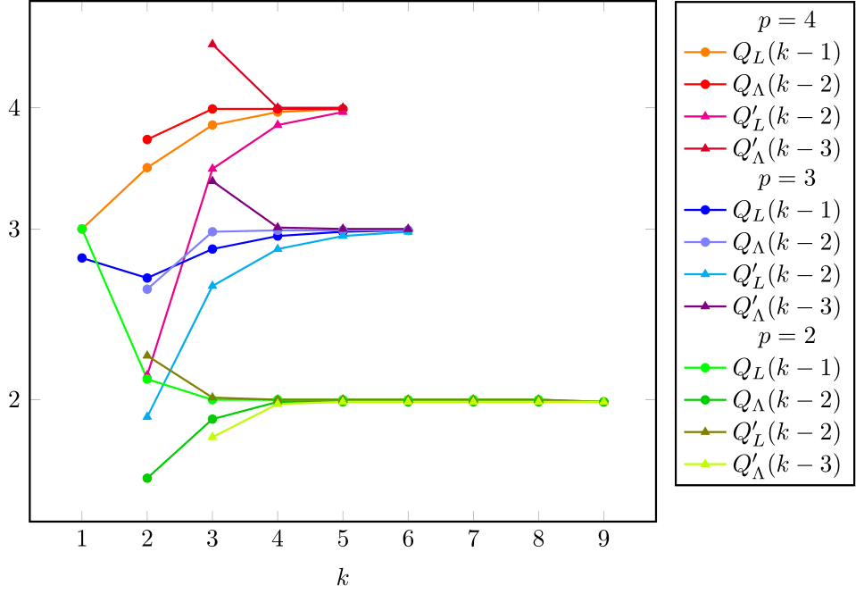
Example 4.9.
Let be a natural given number and consider
By theorem 4.8, we obtain local convergence with -order and .
Let us first deal with . In double precision, for we obtain six nonzero iterates (shown truncated in table 2). In analyzing (shown with the last six decimal digits truncated), we note that is a better approximation than the last one, . This phenomenon may appear even if we increase the precision (see Figure 12).
When and we obtain five nonzero iterates (see 4.11), and is increasingly better.
For and , we obtain four nonzero iterations for the three choices of , and therefore a single meaningful term in computing .
Remark 4.10.
The higher the convergence order, the faster may be reached, and we might end up with fewer distinct terms.
Higher precision is needed in this study. We have chosen to use the Julia language here, which allows not only quadruple precision (digits128, compliant with IEEE 754-2008) but arbitrary precision as well (by using the setprecision command). Some examples are posted at https://github.com/ecatinas/conv-ord and may be easily run online (e.g., by IJulia notebooks running on Binder).232323Such examples may be also performed in MATLAB [58] (by choosing the Advanpix [1] toolbox, which handles arbitrary precision), or in other languages.
In fig. 11 we show the resulting , , , (in order to use only the information available at step ).
We see that all four (computational) convergence orders approach the corresponding ’s, but we cannot clearly distinguish their speed.
In fig. 12 we present and .
Exercise 4.11.
Examining the numerator and denominator in the Newton corrections, give the two different reasons why is in table 2 (when and ). When is realmin or machine epsilon (or both) too large?
(c) -order . The -order is lost with the smoothness of (when ).
Remark 4.13.
Modifying the above example by taking shows that the Newton method may in fact attain any real nonnatural order .
(d) -linear order. This appears for a multiple solution , which is implicitly assumed to be isolated ( in a neighborhood of ).242424Otherwise, an iterative method would not be able to converge to a specific solution we were interested in (take, e.g., the constant function with as the solution set, or , , ). Indeed, if the multiplicity of is ,
| (26) |
(i.e., , ), then (see, e.g., [67, E 10.2-8], [36], [41])
| (27) |
If is known, one may use the Schröder formula [68] to restore the -order :
Exercise 4.14.
(a) Calculate the Newton and Schröder iterates for .
(b) The Schröder iterates are the Newton iterates for .
(e) -sublinear order.
Exercise 4.15.
Let , , . Show that the Newton method converges locally to , with , i.e., -sublinearly.
4.1.4 Convexity
The influence of and the convexity of were first analyzed by Mourraille (1768) [23, sect. 6.3], in an intuitive fashion.
In 1818, Fourier ([38], available on the Internet) gave the condition
| (28) |
which ensures the convergence of the Newton method, provided maintains the monotony and convexity in the interval determined by and . This condition can lead to sided convergence intervals (i.e., not necessarily centered at ).
Clearly, the method may converge even on the whole axis, a result which is more interesting to consider in (cf. the Baluev theorem [66, Thm. 8.3.4]).
Remark 4.16.
(a) By eq. 24, the signs of the errors are periodic with period either (i.e., monotone iterates) or ().
(b) The Fourier condition is sufficient for convergence but not also necessary; the iterates may converge locally (by theorem 4.2) even when eq. 28 does not hold: take, e.g., , , with the signs of errors alternating at each step ().
4.1.5 Attraction Balls
Estimations for as in definition 4.1 are usually given using the condition
| (29) |
The Lipschitz constant of measures the nonlinearity of (i.e., how much the graph of is bent); its exact bound shows this is in accordance with remark 4.5, since
| (30) |
The usual assumptions also require
| (31) |
and the Dennis–Schnabel [32], Rheinboldt [84], and Deuflhard–Potra [35] estimations are, respectively,
| (32) |
where satisfies , , i.e., it can be viewed as a combination of both and (see also [2]).
We note that eq. 32 estimates a small for example 4.6, as is large.
4.1.6 Floating Point Arithmetic
Curious behavior may arise in this setting.
The derivative measures the sensitivity in computing using instead: . This shows that for large , the absolute error in may be amplified. When the relative error in is of interest, the condition number becomes : .
For the relative errors of , the condition numbers are given by [69], [42, sects. 1.2.6 and 5.3]
which show that the relative errors in may be large near a solution .
However, as shown in [42, sects. 1.2.6 and 5.3] and [81, Ex. 2.4, sect. 6.1], the problem of solving an equation has the conditioning number , which is equal to the inverse of the conditioning number for computing .
When (i.e., ) is not small, Shampine, Allen, and Pruess argue that the Newton method is “stable at limiting precision” [89, p. 147], as the Newton corrections are small.
When is small (e.g., is multiple), notable cancellations may appear in computing and prevent the usual graphical interpretation. The (expanded) polynomial of Demmel [28, p. 8] computed in double precision is well known.
Even simpler examples exist: (Sauer [86, p. 45]) and , (Shampine, Allen, and Pruess [89, Fig. 1.2, p. 23]).
not being small is no guarantee that things won’t get weird due to other reasons.
Quiz 4.17 (Wilkinson; see [89, Ex. 4.3]).
Let , , and (here) . Why, in double precision, are the (rounded) Newton iterates: , etc.? Take and compute and .
4.1.7 Nonlinear Systems in
When Newton-type methods are used in practice to solve nonlinear systems in , obtaining high -orders becomes challenging. As the dimension may be huge ( and even higher) the main difficulty resides—having solved the representation of the data in memory252525One can use Newton–Krylov methods, which do not require storage of the matrices , but instead computation of matrix-vector products , further approximated by finite differences [12].—in accurately solving the resulting linear systems eq. 22 at each step. In many practical situations, superlinear convergence may be considered satisfactory.
The most common setting allows the systems eq. 22 to be only approximately solved (the corrections verify , ), leading to the inexact Newton method; its superlinear convergence and the orders were characterized by Dembo, Eisenstat, and Steihaug in [27], the approach being easily extended by us for further sources of perturbation in [14], [17].
The quasi-Newton methods form another important class of Newton-type iterations; they consider approximate Jacobians, in order to produce linear systems that are easier to solve [31]. Their superlinear convergence was characterized by Dennis and Moré [30].
The inexact and quasi-Newton methods are in fact tightly connected models [17].
4.2 The Secant Method
This is a two-step method, requiring ,
| (33) |
but none of the above formulae is recommended for programming (see section 4.2.5).
4.2.1 History
Though nowadays the secant method is usually seen as a Newton-type method with derivatives replaced by finite differences (i.e., a quasi-Newton method) or an inverse interpolatory method, this is not the way it first appeared. The roots of this method can be traced back to approximately the same time as that of the Newton method, the 18th century B.C., found on Babylonian clay tablets and on the Egyptian Rhind Papyrus [23], [70], when it was used as a single iteration for solving linear equations.262626Such equations appear trivial these days, but their solution required ingenuity back then: the decimal system and the zero symbol were used much later, in the 800s (see, e.g., [61, pp. 192–193]). During these times and even later, the terminology for such a noniterated form was “the rule of double false position” (see, e.g., [70]); indeed, two initial “false positions” yield in one iteration the true solution of the linear equation.
Heron of Alexandria [33] approximated the cubic root of by this method (as revealed by Luca and Păvăloiu [57], it turns out that it can be seen as applied equivalently to ).
While reinvented in several cultures (in China,272727Jiuzhang Suanshu (Nine Chapters on the Mathematical Art) [23, sect. 3.3]. India,282828For example, in the work of Madhava’s student Paramesvara [73], [74], [23, sect. 3.4]. Arab countries, and Africa,292929al-Ṭūsī, al-Kāshī, al-Khayyām (see [82], [101], [23, sect. 3.5]). sometimes even for -by- systems of equations), its use as an iterative method was first considered by Cardano (1545), who called it Regula Liberae Positionis [70] (or regula aurea [82, note 5, p. 200]).
4.2.2 Attainable -Orders
The standard convergence result shows the usual convergence with -order given by the golden ratio ; as noted by Papakonstantinou and Tapia [70], this was first obtained by Jeeves in 1958 (in a technical report, published as [48]).
Theorem 4.18 ([68, Chap. 12, sects. 11–12]).
If is simple and , then the secant method has local convergence with -order :
| (34) |
Remark 4.19.
Quiz 4.20.
Remark 4.21.
Higher - (but not necessarily -)orders may be attained.
Theorem 4.22 (Raydan [83]).
If is simple and is the first index such that , then the secant method converges locally with -order given by
and obeys
Moreover, specific results hold in the following cases, noting the attained orders:
-
•
: -order ;
-
•
: exact -order (but not necessarily -order );
-
•
: -order (but not necessarily exact -order ).
Remark 4.23.
When , the secant iterates may have only - but no -order, despite converging to a finite nonzero limit (see 2.25).
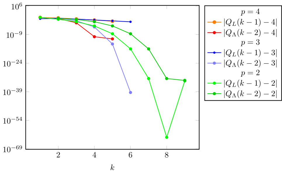
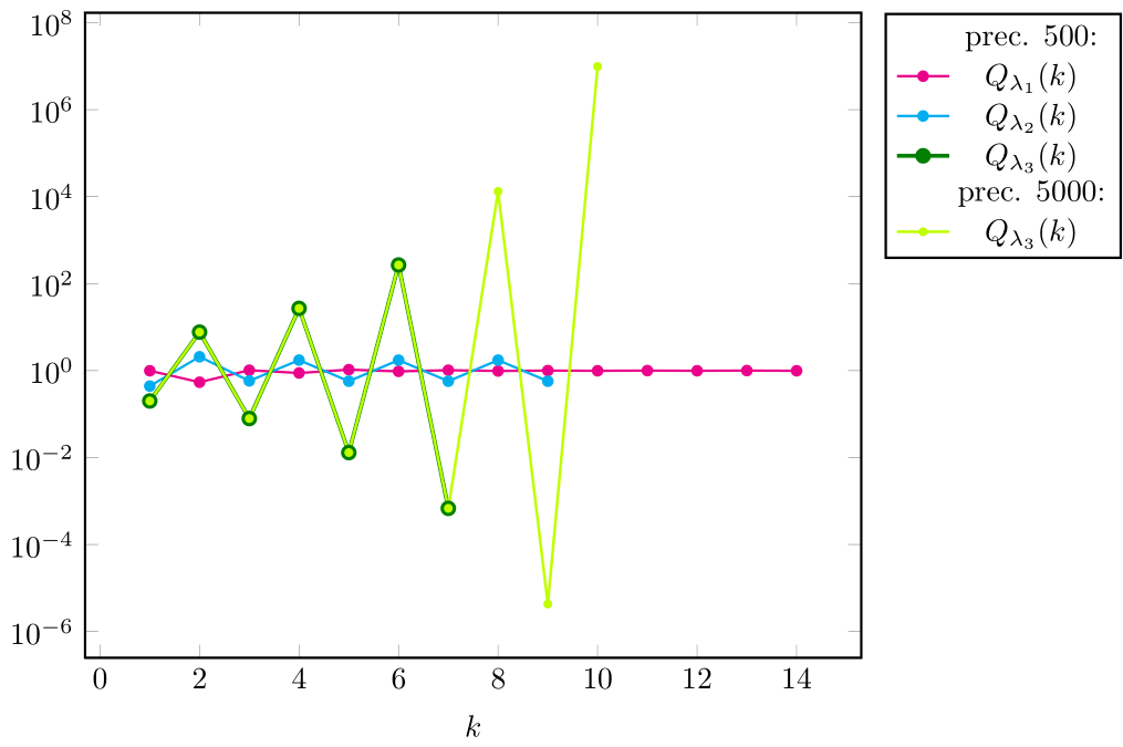
Example 4.24 (cf. [83]).
Let , , , , and compute the secant iterates (by eq. 36).
The assertions of theorem 4.22 are verified in this case, since and , computed using setprecision(500), tend to (see fig. 13).
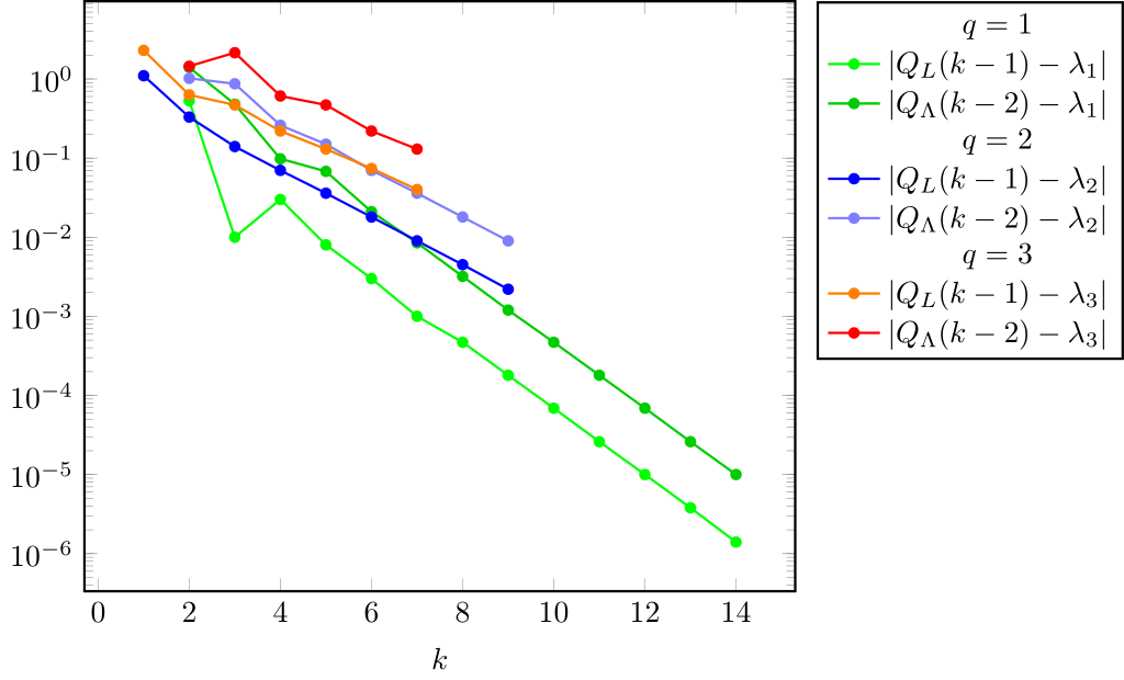
In fig. 14 we plot when and .
We see that tends to .
For oscillates (suggesting , ).
For , tends to infinity (as rigorously proved by Raydan for ). For this particular data it appears that (which remains to be rigorously proved). In order to see it more clearly, we have also used further increased precision (setprecision(5000)), providing confirmation.
When , or do not necessarily hold for any : they do not hold (numerically) for (but they do hold, e.g., for ).
The higher the order, the faster the iterates attain . We see in fig. 14 that setprecision(500) allows iterates when and only iterates when (increased to for setprecision(5000)).
4.2.3 Multiple Solutions
Not only the high orders, but even very local convergence may be lost if is not simple.
4.2.4 Attraction Balls
4.2.5 Floating Point Arithmetic
The two expressions in eq. 33 are not recommended for programming in an ad literam fashion, respectively, at all; indeed, the first one should be written instead as
| (36) |
while the second one can lead, close to , to cancellations when and have the same sign [26, p. 228], [60, p. 4].
Further equivalent formulae are
and (Vandergraft [97, p. 265])
which requires at each step (by swapping the iterates).
It is worth noting, however, that swapping the consecutive iterates in order to obtain leads to iterates that may have a different dynamic than is standard.
The secant method may not be stable at limiting precision, even for large (Shampine, Allen, and Pruess [89, p. 147]), and higher precision may be needed.
4.3 Successive Approximations for Fixed Point Problems
We consider a sufficiently differentiable mapping , , and the fixed point problem
A solution is called a fixed point of ; is further called an attraction fixed point when one has local convergence for the successive approximations
4.3.1 History
Assuming that the computation of with five (decimal) digits is highly improbable in the absence of an iterative method, it is likely that successive approximations date back to at least 1800 B.C. (considering the Newton iterates as particular instances of successive approximations).
Regarding the first use of iterates not connected to the Newton or secant-type iterates, they seem have appeared in the fifth and sixth centuries in India (see Plofker [74]; in this paper the author describes as an example the Brahmasphutasiddhanta of Brahmagupta from the seventh century).
4.3.2 Local Convergence, Attainable -Orders
The first part of the following local convergence result was first obtained by Schröder in 1870 [87]. The extension to mappings in implied the analysis of the eigenvalues of the Jacobian at the fixed point, which is an important topic in numerical analysis.303030Given and the linear system , the following result was called by Ortega [66, p. 118] the fundamental theorem of linear iterative methods: If has a unique solution , then the successive approximations converge to iff the spectral radius is . The standard formulation of the result was first given by Ostrowski in 1957, but Perron had essentially already obtained it in 1929 (see [67, NR 10.1-1]).
Theorem 4.26.
Remark 4.27 (see [67, E 10.1-2]).
Condition is sharp: by considering and taking , is an attraction fixed point, while if , the same fixed point is no longer of attraction.
The higher orders attained are characterized as follows.
Theorem 4.28 (see, e.g., [68, Chap. 4, sect. 10, p. 44], [95], [37]).
Let be an integer and a fixed point of . Then with -order iff
in which case
| (37) |
Example 4.29 ([67, E 10.1-10]).
Any -order is possible: let .
The -sublinear order may be attained too.
Exercise 4.30.
Let and ; then .
The successive approximations are usually regarded as the most general iterations, but actually, they may also be seen as instances of an inexact Newton method [15]; such an approach allows us to study acceleration techniques in a different setting.
4.3.3 Attraction Balls
The following result holds.
Theorem 4.31 ([19]).
Let be an attraction fixed point of for which
Suppose there exist such that is differentiable on with Lipschitz continuous of constant , and denote
| (38) |
Then, , letting we get
which implies that and .
Remark 4.32.
It is important to note that this result does not require to be a contraction on (i.e., ), in contrast to the classical Banach contraction theorem.
The estimate eq. 38 may be sharp in certain cases.
Example 4.33 ([19]).
Let with , , arbitrary, and . Then eq. 38 gives the sharp , since is another fixed point.
We observe that at , which upholds remark 4.32.
Regarding the general case of several dimensions with , we note that the trajectories with high convergence orders are characterized by the zero eigenvalue of and its corresponding eigenvectors (see [16]).
Remark 4.34 ([18, Ex. 2.8]).
definition 4.1 allows a finite number of (regardless of how “small” is chosen to be): take, e.g., , , .
5 Conclusions
Various aspects of convergence orders have been analyzed here, but rather than providing a final view, we see this work as a fresh start; in [21] we pursue the study of the following themes: the characterizations of the -order, the connections between the - and -orders and the big Oh rates, the asymptotic constants (with their immediate computational variants), the convergence orders of the discretization schemes (to mention a few).
6 Answers to Quizzes
1.9: in different windows.
2.7: (a) ; (b) ; (c) , the Fibonacci sequence; (d) .
3.4: unbounded (take ).
4.17: , in double precision.
4.20: the limit is not proved to exist; see also theorem 4.22.
Acknowledgments
I am grateful to two referees for constructive remarks which helped to improve the manuscript, particularly the one who brought the Julia language to my attention; also, I am grateful to my colleagues M. Nechita and I. Boros, as well as to S. Filip for useful suggestions regarding Julia.
References
- [1] Advanpix team, Advanpix, Version 4.7.0.13642, 2020, https://www.advanpix.com/ (accessed 2021/04/07).
- [2] I. K. Argyros and S. George, On a result by Dennis and Schnabel for Newton’s method: Further improvements, Appl. Math. Lett., 55 (2016), pp. 49–53, https://doi.org/10.1016/j.aml.2015.12.003.
- [3] D. F. Bailey, A historical survey of solution by functional iteration, Math. Mag., 62 (1989), pp. 155–166, https://doi.org/10.1080/0025570X.1989.11977428.
- [4] W. A. Beyer, B. R. Ebanks, and C. R. Qualls, Convergence rates and convergence-order profiles for sequences, Acta Appl. Math., 20 (1990), pp. 267–284, https://doi.org/10.1007/bf00049571.
- [5] J. Bezanson, A. Edelman, S. Karpinski, and V. B. Shah, Julia: A fresh approach to numerical computing, SIAM Rev., 59 (2017), pp. 65–98, https://doi.org/10.1137/141000671.
- [6] R. P. Brent, Algorithms for Minimization without Derivatives, Prentice-Hall, Englewood Cliffs, NJ, 1973.
- [7] R. P. Brent, S. Winograd, and P. Wolfe, Optimal iterative processes for root-finding, Numer. Math., 20 (1973), pp. 327–341, https://doi.org/10.1007/bf01402555.
- [8] C. Brezinski, Comparaison des suites convergentes, Rev. Française Inform. Rech. Opér., 5 (1971), pp. 95–99.
- [9] C. Brezinski, Accélération de la Convergence en Analyse Numérique, Springer-Verlag, Berlin, 1977.
- [10] C. Brezinski, Limiting relationships and comparison theorems for sequences, Rend. Circolo Mat. Palermo Ser. II, 28 (1979), pp. 273–280, https://doi.org/10.1007/bf02844100.
- [11] C. Brezinski, Vitesse de convergence d’une suite, Rev. Roumaine Math. Pures Appl., 30 (1985), pp. 403–417.
- [12] P. N. Brown, A local convergence theory for combined inexact-Newton/finite-difference projection methods, SIAM J. Numer. Anal., 24 (1987), pp. 407–434, https://doi.org/10.1137/0724031.
- [13] F. Cajori, Historical note on the Newton-Raphson method of approximation, Amer. Math. Monthly, 18 (1911), pp. 29–32, https://doi.org/10.2307/2973939.
- [14] E. Cătinaş, Inexact perturbed Newton methods and applications to a class of Krylov solvers, J. Optim. Theory Appl., 108 (2001), pp. 543–570, https://doi.org/10.1023/a:1017583307974.
- [15] E. Cătinaş, On accelerating the convergence of the successive approximations method, Rev. Anal. Numér. Théor. Approx., 30 (2001), pp. 3–8, https://ictp.acad.ro/accelerating-convergence-successive-approximations-method/ (accessed 2021/04/07).
- [16] E. Cătinaş, On the superlinear convergence of the successive approximations method, J. Optim. Theory Appl., 113 (2002), pp. 473–485, https://doi.org/10.1023/a:1015304720071.
- [17] E. Cătinaş, The inexact, inexact perturbed and quasi-Newton methods are equivalent models, Math. Comp., 74 (2005), pp. 291–301, https://doi.org/10.1090/s0025-5718-04-01646-1.
- [18] E. Cătinaş, Newton and Newton-type Methods in Solving Nonlinear Systems in , Risoprint, Cluj-Napoca, Romania, 2007, https://ictp.acad.ro/methods-of-newton-and-newton-krylov-type/ (accessed on 2021/6/9).
- [19] E. Cătinaş, Estimating the radius of an attraction ball, Appl. Math. Lett., 22 (2009), pp. 712–714, https://doi.org/10.1016/j.aml.2008.08.007.
- [20] E. Cătinaş, A survey on the high convergence orders and computational convergence orders of sequences, Appl. Math. Comput., 343 (2019), pp. 1–20, https://doi.org/10.1016/j.amc.2018.08.006.
- [21] E. Cătinaş, How Many Steps Still Left to *? Part II. Newton Iterates without and , manuscript, 2020.
- [22] A. Cauchy, Sur la determination approximative des racines d’une equation algebrique ou transcendante, Oeuvres Complete (II) 4, Gauthier-Villars, Paris, 1899, 23 (1829), pp. 573–609, http://iris.univ-lille.fr/pdfpreview/bitstream/handle/1908/4026/41077-2-4.pdf?sequence=1 (accessed 2021/04/07).
- [23] J.-L. Chabert, ed., A History of Algorithms. From the Pebble to the Microchip, Springer-Verlag, Berlin, 1999.
- [24] J. Chen and I. K. Argyros, Improved results on estimating and extending the radius of an attraction ball, Appl. Math. Lett., 23 (2010), pp. 404–408, https://doi.org/10.1016/j.aml.2009.11.007.
- [25] A. R. Conn, N. I. M. Gould, and P. L. Toint, Trust-Region Methods, SIAM, Philadelphia, PA, 2000, https://doi.org/10.1137/1.9780898719857.
- [26] G. Dahlquist and Å. Björk, Numerical Methods, Dover, Mineola, NY, 1974.
- [27] R. S. Dembo, S. C. Eisenstat, and T. Steihaug, Inexact Newton methods, SIAM J. Numer. Anal., 19 (1982), pp. 400–408, https://doi.org/10.1137/0719025.
- [28] J. W. Demmel, Applied Numerical Linear Algebra, SIAM, Philadelphia, PA, 1997, https://doi.org/10.1137/1.9781611971446.
- [29] J. E. Dennis, On Newton-like methods, Numer. Math., 11 (1968), pp. 324–330, https://doi.org/10.1007/bf02166685.
- [30] J. E. Dennis, Jr., and J. J. Moré, A characterization of superlinear convergence and its application to quasi-Newton methods, Math. Comp., 28 (1974), pp. 549–560, https://doi.org/10.1090/s0025-5718-1974-0343581-1.
- [31] J. E. Dennis, Jr., and J. J. Moré, Quasi-Newton methods, motivation and theory, SIAM Rev., 19 (1977), pp. 46–89, https://doi.org/10.1137/1019005.
- [32] J. E. Dennis, Jr., and R. B. Schnabel, Numerical Methods for Unconstrained Optimization and Nonlinear Equations, SIAM, Philadelphia, PA, 1996, https://doi.org/10.1137/1.9781611971200.
- [33] G. Deslauries and S. Dubuc, Le calcul de la racine cubique selon Héron, Elem. Math., 51 (1996), pp. 28–34, http://eudml.org/doc/141587 (accessed 2020/02/18).
- [34] P. Deuflhard, Newton Methods for Nonlinear Problems. Affine Invariance and Adaptive Algorithms, Springer-Verlag, Heidelberg, 2004.
- [35] P. Deuflhard and F. A. Potra, Asymptotic mesh independence of Newton–Galerkin methods via a refined Mysovskii theorem, SIAM J. Numer. Anal., 29 (1992), pp. 1395–1412, https://doi.org/10.1137/0729080.
- [36] P. Díez, A note on the convergence of the secant method for simple and multiple roots, Appl. Math. Lett., 16 (2003), pp. 1211–1215, https://doi.org/10.1016/s0893-9659(03)90119-4.
- [37] F. Dubeau and C. Gnang, Fixed point and Newton’s methods for solving a nonlinear equation: From linear to high-order convergence, SIAM Rev., 56 (2014), pp. 691–708, https://doi.org/10.1137/130934799.
- [38] J. Fourier, Question d’analyse algébrique, Bull. Sci. Soc. Philo., 67 (1818), pp. 61–67, http://gallica.bnf.fr/ark:/12148/bpt6k33707/f248.item (accessed 2021-04-07).
- [39] W. Gautschi, Numerical Analysis, 2nd ed., Birkhäuser/Springer, New York, 2011, https://doi.org/10.1007/978-0-8176-8259-0.
- [40] M. Grau-Sánchez, M. Noguera, and J. M. Gutiérrez, On some computational orders of convergence, Appl. Math. Lett., 23 (2010), pp. 472–478, https://doi.org/10.1016/j.aml.2009.12.006.
- [41] A. Greenbaum and T. P. Chartier, Numerical Methods. Design, Analysis, and Computer Implementation of Algorithms, Princeton University Press, Princeton, NJ, 2012.
- [42] M. T. Heath, Scientific Computing. An Introductory Survey, 2nd ed., SIAM, Philadelphia, PA, 2018, https://doi.org/10.1137/1.9781611975581.
- [43] M. Heinkenschloss, Scientific Computing. An Introductory Survey, Rice University, Houston, TX, 2018.
- [44] J. Herzberger and L. Metzner, On the Q-order of convergence for coupled sequences arising in iterative numerical processes, Computing, 57 (1996), pp. 357–363, https://doi.org/10.1007/BF02252254.
- [45] N. J. Higham, Accuracy and Stability of Numerical Algorithms, 2nd ed., SIAM, Philadelphia, PA, 2002, https://doi.org/10.1137/1.9780898718027.
- [46] M. Igarashi and T. J. Ypma, Empirical versus asymptotic rate of convergence of a class of methods for solving a polynomial equation, J. Comput. Appl. Math., 82 (1997), pp. 229–237, https://doi.org/10.1016/s0377-0427(97)00077-0.
- [47] L. O. Jay, A note on Q-order of convergence, BIT, 41 (2001), pp. 422–429, https://doi.org/10.1023/A:1021902825707.
- [48] T. A. Jeeves, Secant modification of Newton’s method, Commun. ACM, 1 (1958), pp. 9–10, https://doi.org/10.1145/368892.368913.
- [49] V. J. Katz, A History of Mathematics. An Introduction, 2nd ed., Addison-Wesley, 1998.
- [50] C. T. Kelley, Iterative Methods for Linear and Nonlinear Equations, SIAM, Philadelphia, PA, 1995, https://doi.org/10.1137/1.9781611970944.
- [51] C. T. Kelley, Iterative Methods for Optimization, SIAM, Philadelphia, PA, 1999, https://doi.org/10.1137/1.9781611970920.
- [52] E. S. Kennedy and W. R. Transue, A medieval iterative algorism, Amer. Math. Monthly, 63 (1956), pp. 80–83, https://doi.org/10.1080/00029890.1956.11988762.
- [53] D. E. Knuth, Big Omicron and big Omega and big Theta, ACM SIGACT News, 8 (1976), pp. 18–24, https://doi.org/10.1145/1008328.1008329.
- [54] D. E. Knuth, The TeXbook, Addison-Wesley, 1984.
- [55] N. Kollerstrom, Thomas Simpson and Newton’s method of approximation: An enduring myth, British J. History Sci., 25 (1992), pp. 347–354, https://doi.org/10.1017/s0007087400029150.
- [56] K. Liang, Homocentric convergence ball of the secant method, Appl. Math. Chin. Univ., 22 (2007), pp. 353–365, https://doi.org/10.1007/s11766-007-0313-3.
- [57] D. Luca and I. Păvăloiu, On the Heron’s method for approximating the cubic root of a real number, Rev. Anal. Numér. Théor. Approx., 26 (1997), pp. 103–108, https://ictp.acad.ro/jnaat/journal/article/view/1997-vol26-nos1-2-art15 (accessed 2021-04-07).
- [58] Mathworks, MATLAB, Version 2019b, 2019, http://www.mathworks.com (accessed 2021/04/07).
- [59] J. M. McNamee, Numerical Methods for Roots of Polynomials, Part I, Elsevier, Amsterdam, 2007.
- [60] J. M. McNamee and V. Y. Pan, Numerical Methods for Roots of Polynomials, Part II, Elsevier, Amsterdam, 2013.
- [61] U. C. Merzbach and C. B. Boyer, A History of Mathematics, 3rd ed., John Wiley & Sons, 2011.
- [62] J.-M. Muller, N. Brunie, F. de Dinechin, C.-P. Jeannerod, M. Joldes, V. Lefèvre, G. Melquiond, N. Revol, and S. Torres, Handbook of Floating-Point Arithmetic, 2nd ed., Springer, New York, 2018, https://doi.org/10.1007/978-3-319-76526-6.
- [63] A. S. Nemirovsky and D. B. Yudin, Problem Complexity and Method Efficiency in Optimization, Wiley, 1983.
- [64] A. Neumaier, Introduction to Numerical Analysis, Cambridge University Press, 2001.
- [65] J. Nocedal and S. J. Wright, Numerical Optimization, 2nd ed., Springer, New York, 2006, https://doi.org/10.1007/978-0-387-40065-5.
- [66] J. M. Ortega, Numerical Analysis. A Second Course, SIAM, Philadelphia, PA, 1990, https://doi.org/10.1137/1.9781611971323.
- [67] J. M. Ortega and W. C. Rheinboldt, Iterative Solution of Nonlinear Equations in Several Variables, SIAM, Philadelphia, PA, 2000, https://doi.org/10.1137/1.9780898719468.
- [68] A. M. Ostrowski, Solution of Equations and Systems of Equations, 2nd ed., Academic Press, New York, 1966; 3rd ed., 1972.
- [69] M. L. Overton, Numerical Computing with IEEE Floating Point Arithmetic, SIAM, Philadelphia, PA, 2001, https://doi.org/10.1137/1.9780898718072.
- [70] J. M. Papakonstantinou and R. A. Tapia, Origin and evolution of the secant method in one dimension, Amer. Math. Monthly, 120 (2013), pp. 500–518, https://doi.org/10.4169/amer.math.monthly.120.06.500.
- [71] I. Păvăloiu, Sur l’ordre de convergence des méthodes d’itération, Mathematica, 23 (46) (1981), pp. 261–265, https://ictp.acad.ro/convergence-order-iterative-methods/.
- [72] I. Păvăloiu, Optimal algorithms concerning the solving of equations by interpolation, in Research on Theory of Allure, Approximation, Convexity and Optimization, Editura Srima, 1999, pp. 222–248, http://ictp.acad.ro/optimal-algorithms-concerning-solving-equations-interpolation/ (accessed 2021-04-07).
- [73] K. Plofker, An example of the secant method of iterative approximation in a fifteenth-century Sanskrit text, Historia Math., 23 (1996), pp. 246–256, https://doi.org/10.1006/hmat.1996.0026.
- [74] K. Plofker, Use and transmission of iterative approximations in India and the Islamic World, in From China to Paris: 2000 Years Transmission of Mathematical Ideas, Y. Dold-Samplonius, J. W. Dauben, M. Folkerts, and B. Van Dalen, eds., Franz Steiner Verlag Wiesbaden GmbH, Stuttgart, 2002, pp. 167–186.
- [75] E. Polak, Optimization. Algorithms and Consistent Approximations, Springer-Verlag, New York, 1997.
- [76] F. A. Potra, On Q-order and R-order of convergence, J. Optim. Theory Appl., 63 (1989), pp. 415–431, https://doi.org/10.1007/bf00939805.
- [77] F. A. Potra, Q-superlinear convergence of the iterates in primal-dual interior-point methods, Math. Program. Ser. A, 91 (2001), pp. 99–115, https://doi.org/10.1007/s101070100230.
- [78] F. A. Potra, A superquadratic version of Newton’s method, SIAM J. Numer. Anal., 55 (2017), pp. 2863–2884, https://doi.org/10.1137/17M1121056.
- [79] F. A. Potra and V. Pták, Nondiscrete Induction and Iterative Processes, Pitman, Boston, MA, 1984.
- [80] F. A. Potra and R. Sheng, A path following method for LCP with superlinearly convergent iteration sequence, Ann. Oper. Res., 81 (1998), pp. 97–114, https://doi.org/10.1023/A:1018942131812.
- [81] A. Quarteroni, R. Sacco, and F. Saleri, Numerical Mathematics, Springer, Berlin, 2007.
- [82] R. Rashed, The Development of Arabic Mathematics: Between Arithmetic and Algebra, Stud. Philos. Sci. 156, Springer, Boston, MA, 1994.
- [83] M. Raydan, Exact order of convergence of the secant method, J. Optim. Theory Appl., 78 (1993), pp. 541–551, https://doi.org/10.1007/BF00939881.
- [84] W. C. Rheinboldt, An adaptive continuation process for solving systems of nonlinear equations, in Mathematical Models and Numerical Methods, Banach Ctr. Publ. 3, Polish Academy of Science, 1977, pp. 129–142, https://doi.org/10.4064/-3-1-129-142.
- [85] W. C. Rheinboldt, Methods for Solving Systems of Nonlinear Equations, 2nd ed., SIAM, Philadelphia, PA, 1998, https://doi.org/10.1137/1.9781611970012.
- [86] T. Sauer, Numerical Analysis, 2nd ed., Pearson, Boston, MA, 2012.
- [87] E. Schröder, Ueber unendlich viele Algorithmen zur Auflösung der Gleichungen, Math. Ann., 2 (1870), pp. 317–365, https://doi.org/10.1007/bf01444024; available as On Infinitely Many Algorithms for Solving Equations, Tech reports TR–92–121 and TR–2990, Institute for Advanced Computer Studies, University of Maryland, 1992; translated by G. W. Stewart.
- [88] H. Schwetlick, Numerische Lösung Nichtlinearer Gleichungen, VEB, Berlin, 1979.
- [89] L. F. Shampine, R. C. Allen, Jr., and S. Pruess, Fundamentals of Numerical Computing, John Wiley and Sons, New York, 1997.
- [90] T. Steihaug, Computational science in the eighteenth century. Test cases for the methods of Newton, Raphson, and Halley: to , Numer. Algorithms, 83 (2020), pp. 1259–1275, https://doi.org/10.1007/s11075-019-00724-8.
- [91] E. Süli and D. Mayers, An Introduction to Numerical Analysis, Cambridge University Press, Cambridge, UK, 2003.
- [92] T. Tantau, The tikz and pgf Packages. Manual for Version b--gffccd, https://github.com/pgf-tikz/pgf.
- [93] R. A. Tapia, J. E. Dennis, Jr., and J. P. Schäfermeyer, Inverse, shifted inverse, and Rayleigh quotient iteration as Newton’s method, SIAM Rev., 60 (2018), pp. 3–55, https://doi.org/10.1137/15M1049956.
- [94] R. A. Tapia and D. L. Whitley, The projected Newton method has order for the symmetric eigenvalue problem, SIAM J. Numer. Anal., 25 (1988), pp. 1376–1382, https://doi.org/10.1137/0725079.
- [95] J. F. Traub, Iterative Methods for the Solutions of Equations, Prentice Hall, Englewood Cliffs, NJ, 1964.
- [96] E. E. Tyrtyshnikov, A Brief Introduction to Numerical Analysis, Birkhäuser/Springer, New York, 1997.
- [97] J. S. Vandergraft, Introduction to Numerical Computations, 2nd ed., Academic Press, New York, 1983.
- [98] H. F. Walker, An approach to continuation using Krylov subspace methods, in Computational Science in the 21st Century, J. Periaux, ed., John Wiley and Sons, 1997, pp. 72–81.
- [99] S. J. Wright, Primal-Dual Interior-Point Methods, SIAM, Philadelphia, PA, 1997, https://doi.org/10.1137/1.9781611971453.
- [100] S. J. Wright, Optimization algorithms for data analysis, in The Mathematics of Data, IAS/Park City Math. Ser. 25, AMS, Providence, RI, 2018, pp. 49–97.
- [101] T. J. Ypma, Historical development of the Newton–Raphson method, SIAM Rev., 37 (1995), pp. 531–551, https://doi.org/10.1137/1037125.
[1] Advanpix team, Advanpix, Version 4.7.0.13642, 2020, https://www.advanpix.com/ (accessed 2020/03/22). (Cited on pp. 4, 26)
[2] I. K. Argyros and S. George, On a result by Dennis and Schnabel for Newton’s method: Further improvements, Appl. Math. Lett., 55 (2016), pp. 49-53, https://doi.org/10.1016/j.aml.2015.12.003. (Cited on p. 28)
[3] D. F. Bailey, A historical survey of solution by functional iteration, Math. Mag., 62 (1989), pp. 155-166, https://doi.org/10.1080/0025570X.1989.11977428. (Cited on pp. 7, 21, 34)
[4] W. A. Beyer, B. R. Ebanks, and C. R. Qualls, Convergence rates and convergence-order profiles for sequences, Acta Appl. Math., 20 (1990), pp. 267-284, https://doi.org/10.1007/bf00049571. (Cited on pp. 8, 9, 11, 14, 17, 19, 21)
[5] J. Bezanson, A. Edelman, S. Karpinski, and V. B. Shah, Julia: A fresh approach to numerical computing, SIAM Rev., 59 (2017), pp. 65-98, https://doi.org/10.1137/141000671. (Cited on p. 4)
[6] R. P. Brent, Algorithms for Minimization without Derivatives, Prentice-Hall, Englewood Cliffs, NJ, 1973. (Cited on p. 11)
[7] R. P. Brent, S. Winograd, and P. Wolfe, Optimal iterative processes for root-finding, Numer. Math., 20 (1973), pp. 327-341, https://doi.org/10.1007/bf01402555. (Cited on pp. 13, 15)
[8] C. Brezinski, Comparaison des suites convergentes, Rev. Franҫaise Inform. Rech. Oper., 5 (1971), pp. 95-99. (Cited on pp. 13, 14)
[9] C. Brezinski, Acceleration de la Convergence en Analyse Numerique, Springer-Verlag, Berlin, 1977. (Cited on pp. 2, 13, 14)
[10] C. Brezinski, Limiting relationships and comparison theorems for sequences, Rend. Circolo Mat. Palermo Ser. II, 28 (1979), pp. 273-280, https://doi.org/10.1007/bf02844100. (Cited on p. 19)
[11] C. Brezinski, Vitesse de convergence d’une suite, Rev. Roumaine Math. Pures Appl., 30 (1985), pp. 403-417. (Cited on pp. 11, 13, 18)
[12] P. N. Brown, A local convergence theory for combined inexact-Newton/finite-difference projection methods, SIAM J. Numer. Anal., 24 (1987), pp. 407-434, https://doi.org/10.1137/0724031. (Cited on p. 29)
[13] F. Cajori, Historical note on the Newton-Raphson method of approximation, Amer. Math. Monthly, 18 (1911), pp. 29-32, https://doi.org/10.2307/2973939. (Cited on pp. 22, 23)
[14] A. Cauchy, Sur la determination approximative des racines d’une equation algebrique ou transcendante, Oeuvres Complete (II) 4, Gauthier-Villars, Paris, 1899, 23 (1829), pp. 573-609, http://iris.univ-lille1.fr/pdfpreview/bitstream/handle/1908/4026/41077-2-4.pdf?sequence=1 (accessed 2019/02/01). (Cited on pp. 21, 23)
[15] J.-L. Chabert, ed., A History of Algorithms. From the Pebble to the Microchip, Springer Verlag, Berlin, 1999. (Cited on pp. 21, 22, 23, 28, 30, 34)
[16] J. Chen and I. K. Argyros, Improved results on estimating and extending the radius of an attraction ball, Appl. Math. Lett., 23 (2010), pp. 404-408, https://doi.org/10.1016/j.aml.2009.11.007. (Cited on p. 35)
[17] A. R. Conn, N. I. M. Gould, and P. L. Toint, Trust-Region Methods, SIAM, Philadelphia, PA, 2000, https://doi.org/10.1137/1.9780898719857. (Cited on pp. 14, 17)
[18] E. Catinas, Inexact perturbed Newton methods and applications to a class of Krylov solvers, J. Optim. Theory Appl., 108 (2001), pp. 543-570, https://doi.org/10.1023/a:1017583307974. (Cited on p. 29)
[19] E. Catinas, On accelerating the convergence of the successive approximations method, Rev. Anal. Numer. Theor. Approx., 30 (2001), pp. 3-8, https://ictp.acad.ro/acceleratingconvergence-successive-approximations-method/ (accessed 20/10/10). (Cited on p. 34)
[20] E. Catinas, On the superlinear convergence of the successive approximations method, J. Optim. Theory Appl., 113 (2002), pp. 473-485, https://doi.org/10.1023/a:1015304720071. (Cited on p. 35)
[21] E. Catinas, The inexact, inexact perturbed and quasi-Newton methods are equivalent models, Math. Comp., 74 (2005), pp. 291-301, https://doi.org/10.1090/s0025-5718-04-01646-1. (Cited on p. 29)
[22] E. Catinas, Newton and Newton-type Methods in Solving Nonlinear Systems in RN , Risoprint, Cluj-Napoca, 2007. (Cited on p. 35)
[23] E. Catinas, Estimating the radius of an attraction ball, Appl. Math. Lett., 22 (2009), pp. 712-714, https://doi.org/10.1016/j.aml.2008.08.007. (Cited on p. 35)
[24] E. Catinas, A survey on the high convergence orders and computational convergence orders of sequences, Appl. Math. Comput., 343 (2019), pp. 1-20, https://doi.org/10.1016/j.amc.2018.08.006. (Cited on pp. 7, 8, 10, 11, 12, 14, 15, 16, 17, 18, 20, 21)
[25] E. Catinas, How Many Steps Still Left to x*? Part II. Newton iterates without f and f’, manuscript, 2020. (Cited on pp. 24, 35)
[26] G. Dahlquist and A. Bjork, Numerical Methods, Dover, Mineola, NY, 1974. (Cited on p. 33)
[27] R. S. Dembo, S. C. Eisenstat, and T. Steihaug, Inexact Newton methods, SIAM J. Numer. Anal., 19 (1982), pp. 400-408, https://doi.org/10.1137/0719025. (Cited on p. 29)
[28] J. W. Demmel, Applied Numerical Linear Algebra, SIAM, Philadelphia, PA, 1997, https://doi.org/10.1137/1.9781611971446. (Cited on pp. 3, 29)
[29] J. E. Dennis, On Newton-like methods, Numer. Math., 11 (1968), pp. 324-330, https://doi.org/10.1007/bf02166685. (Cited on p. 17)
[30] J. E. Dennis, Jr., and J. J. More, A characterization of superlinear convergence and its application to quasi-Newton methods, Math. Comp., 28 (1974), pp. 549-560, https://doi.org/10.1090/s0025-5718-1974-0343581-1. (Cited on pp. 19, 29)
[31] J. E. Dennis, Jr., and J. J. More, Quasi-Newton methods, motivation and theory, SIAM Rev., 19 (1977), pp. 46-89, https://doi.org/10.1137/1019005. (Cited on pp. 27, 29)
[32] J. E. Dennis, Jr., and R. B. Schnabel, Numerical Methods for Unconstrained Optimization and Nonlinear Equations, SIAM, Philadelphia, PA, 1996, https://doi.org/10.1137/1.9781611971200. (Cited on pp. 15, 28)
[33] G. Deslauries and S. Dubuc, Le calcul de la racine cubique selon Heron, Elem. Math., 51 (1996), pp. 28-34, http://eudml.org/doc/141587 (accessed 2020/02/18). (Cited on p. 30)
[34] P. Deuflhard, Newton Methods for Nonlinear Problems. Affine Invariance and Adaptive Algorithms, Springer-Verlag, Heidelberg, 2004. (Cited on pp. 23, 24)
[35] P. Deuflhard and F. A. Potra, Asymptotic mesh independence of Newton-Galerkin methods via a refined Mysovskii theorem, SIAM J. Numer. Anal., 29 (1992), pp. 1395-1412, https://doi.org/10.1137/0729080. (Cited on p. 28)
[36] P. Diez, A note on the convergence of the secant method for simple and multiple roots, Appl. Math. Lett., 16 (2003), pp. 1211-1215, https://doi.org/10.1016/s0893-9659(03)90119-4. (Cited on pp. 27, 31)
[37] F. Dubeau and C. Gnang, Fixed point and Newton’s methods for solving a nonlinear equation: From linear to high-order convergence, SIAM Rev., 56 (2014), pp. 691-708, https://doi.org/10.1137/130934799. (Cited on pp. 25, 34)
[38] J. Fourier, Question d’analyse algebrique, Bull. Sci. Soc. Philo., 67 (1818), pp. 61-67, http://gallica.bnf.fr/ark:/12148/bpt6k33707/f248.item (accessed 2018-02-23). (Cited on pp. 7, 28)
[39] W. Gautschi, Numerical Analysis, 2nd ed., Birkhauser/Springer, New York, 2011, https://doi.org/10.1007/978-0-8176-8259-0. (Cited on p. 23)
[40] A. Greenbaum and T. P. Chartier, Numerical Methods. Design, Analysis, and Computer Implementation of Algorithms, Princeton University Press, Princeton, NJ, 2012. (Cited on pp. 23, 27, 31)
[41] M. T. Heath, Scientific Computing. An Introductory Survey, 2nd ed., SIAM, Philadelphia, PA, 2018, https://doi.org/10.1137/1.9781611975581. (Cited on pp. 9, 29)
[42] M. Heinkenschloss, Scientific Computing. An Introductory Survey, Rice University, Houston, TX, 2018. (Cited on pp. 3, 15, 19)
[43] J. Herzberger and L. Metzner, On the Q-order of convergence for coupled sequences arising in iterative numerical processes, Computing, 57 (1996), pp. 357-363, https://doi.org/10.1007/BF02252254. (Cited on p. 13)
[44] N. J. Higham, Accuracy and Stability of Numerical Algorithms, 2nd ed., SIAM, Philadelphia, PA, 2002, https://doi.org/10.1137/1.9780898718027. (Cited on p. 3)
[45] M. Igarashi and T. J. Ypma, Empirical versus asymptotic rate of convergence of a class of methods for solving a polynomial equation, J. Comput. Appl. Math., 82 (1997), pp. 229-237, https://doi.org/10.1016/s0377-0427(97)00077-0. (Cited on p. 25)
[46] L. O. Jay, A note on Q-order of convergence, BIT, 41 (2001), pp. 422-429, https://doi.org/10.1023/A:1021902825707. (Cited on pp. 5, 11, 12, 17)
[47] T. A. Jeeves, Secant modification of Newton’s method, Commun. ACM, 1 (1958), pp. 9-10, https://doi.org/10.1145/368892.368913. (Cited on pp. 11, 30)
[48] V. J. Katz, A History of Mathematics. An Introduction, 2nd ed., Addison-Wesley, 1998. (Cited on p. 21)
[49] C. T. Kelley, Iterative Methods for Linear and Nonlinear Equations, SIAM, Philadelphia, PA, 1995, https://doi.org/10.1137/1.9781611970944. (Cited on pp. 5, 10, 17)
[50] C. T. Kelley, Iterative Methods for Optimization, SIAM, Philadelphia, PA, 1999, https://doi.org/10.1137/1.9781611970920. (Cited on pp. 15, 17)
[51] E. S. Kennedy and W. R. Transue, A medieval iterative algorism, Amer. Math. Monthly, 63 (1956), pp. 80-83, https://doi.org/10.1080/00029890.1956.11988762. (Cited on p. 34)
[52] D. E. Knuth, Big Omicron and big Omega and big Theta, ACM SIGACT News, 8 (1976), pp. 18-24, https://doi.org/10.1145/1008328.1008329. (Cited on pp. 2, 14)
[53] D. E. Knuth, The TeXbook, Addison-Wesley, 1984. (Cited on p. 4)
[54] N. Kollerstrom, Thomas Simpson and Newton’s method of approximation: an enduring myth, British J. History Sci., 25 (1992), pp. 347-354, https://doi.org/10.1017/s0007087400029150. (Cited on pp. 22, 23)
[55] K. Liang, Homocentric convergence ball of the secant method, Appl. Math. Chin. Univ., 22 (2007), pp. 353–365, https://doi.org/10.1007/s11766-007-0313-3. (Cited on p. 33)
[56] D. Luca and I. Pavaloiu, On the Heron’s method for approximating the cubic root of a real number, Rev. Anal. Numer. Theor. Approx., 26 (1997), pp. 103-108, https://ictp.acad.ro/jnaat/journal/article/view/1997-vol26-nos1-2-art15 (accessed 2020-03-21). (Cited on p. 30)
[57] M. Grau-Sanchez, M. Noguera, and J. M. Gutierrez, On some computational orders of convergence, Appl. Math. Lett., 23 (2010), pp. 472-478, https://doi.org/10.1016/j.aml.2009.12.006. (Cited on p. 20)
[58] Mathworks, MATLAB, Version 2019b, 2019, http://www.mathworks.com (accessed 2019/12/12). (Cited on pp. 4, 26)
[59] J. M. McNamee, Numerical Methods for Roots of Polynomials, Part I, Elsevier, Amsterdam, 2007. (Cited on p. 23)
[60] J. M. McNamee and V. Y. Pan, Numerical Methods for Roots of Polynomials, Part II, Elsevier, Amsterdam, 2013. (Cited on pp. 28, 33)
[61] U. C. Merzbach and C. B. Boyer, A History of Mathematics, 3rd ed., John Wiley & Sons, 2011. (Cited on p. 30)
[62] J.-M. Muller, N. Brunie, F. de Dinechin, C.-P. Jeannerod, M. Joldes, V. Lefevre, G. Melquiond, N. Revol, and S. Torres, Handbook of Floating-Point Arithmetic, 2nd ed., Springer, New York, 2018, https://doi.org/10.1007/978-3-319-76526-6. (Cited on pp. 22, 24)
[63] A. S. Nemirovsky and D. B. Yudin, Problem Complexity and Method Efficiency in Optimization, Wiley, 1983. (Cited on p. 15)
[64] A. Neumaier, Introduction to Numerical Analysis, Cambridge University Press, 2001. (Cited on pp. 31, 33)
[65] J. Nocedal and S. J. Wright, Numerical Optimization, 2nd ed., Springer, New York, 2006, https://doi.org/10.1007/978-0-387-40065-5. (Cited on pp. 8, 17)
[66] J. M. Ortega, Numerical Analysis. A Second Course, SIAM, Philadelphia, PA, 1990, https://doi.org/10.1137/1.9781611971323. (Cited on pp. 28, 34)
[67] J. M. Ortega and W. C. Rheinboldt, Iterative Solution of Nonlinear Equations in Several Variables, SIAM, Philadelphia, PA, 2000, https://doi.org/10.1137/1.9780898719468. (Cited on pp. 8, 10, 11, 14, 15, 16, 18, 21, 27, 34)
[68] A. M. Ostrowski, Solution of Equations and Systems of Equations, 2nd ed., Academic Press, New York, 1966; 3rd ed., 1972. (Cited on pp. 27, 30, 34)
[69] M. L. Overton, Numerical Computing with IEEE Floating Point Arithmetic, SIAM, Philadelphia, PA, 2001, https://doi.org/10.1137/1.9780898718072. (Cited on pp. 3, 29)
[70] J. M. Papakonstantinou and R. A. Tapia, Origin and evolution of the secant method in one dimension, Amer. Math. Monthly, 120 (2013), pp. 500-518, https://doi.org/10.4169/amer.math.monthly.120.06.500. (Cited on p. 30)
[71] K. Plofker, An example of the secant method of iterative approximation in a fifteenth century sanskrit text, Historia Math., 23 (1996), pp. 246-256, https://doi.org/10.1006/hmat.1996.0026. (Cited on pp. 30, 34)
[72] K. Plofker, Use and transmission of iterative approximations in India and the Islamic World, in From China to Paris: 2000 Years Transmission of Mathematical Ideas, Y. Dold-Samplonius, J. W. Dauben, M. Folkerts, and B. Van Dalen, eds., Franz Steiner Verlag Wiesbaden GmbH, Stuttgart, 2002, pp. 167-186. (Cited on pp. 21, 22, 30, 34)
[73] E. Polak, Optimization. Algorithms and Consistent Approximations, Springer-Verlag, New York, 1997. (Cited on pp. 5, 11, 15, 19)
[74] F. A. Potra, On Q-order and R-order of convergence, J. Optim. Theory Appl., 63 (1989), pp. 415-431, https://doi.org/10.1007/bf00939805. (Cited on pp. 8, 11, 13, 14, 15, 16, 17, 18, 21) [75] F. A. Potra, Q-superlinear convergence of the iterates in primal-dual interior-point methods, Math. Program. Ser. A, 91 (2001), pp. 99-115, https://doi.org/10.1007/s101070100230. (Cited on p. 15)
[76] F. A. Potra, A superquadratic version of Newton’s method, SIAM J. Numer. Anal., 55 (2017), pp. 2863-2884, https://doi.org/10.1137/17M1121056. (Cited on p. 13)
[77] F. A. Potra and V. Ptak, Nondiscrete Induction and Iterative Processes, Pitman, Boston, MA, 1984. (Cited on pp. 8, 11, 13, 15, 19)
[78] F. A. Potra and R. Sheng, A path following method for LCP with superlinearly convergent iteration sequence, Ann. Oper. Res., 81 (1998), pp. 97-11, https://doi.org/10.1023/A:1018942131812. (Cited on p. 14)
[79] I. Pavaloiu, Sur l’ordre de convergence des methodes d’iteration, Mathematica, 23(46) (1981), pp. 261-272, https://doi.org/10.1007/BF02576543. (Cited on p. 14)
[80] I. Pavaloiu, Optimal algorithms concerning the solving of equations by interpolation, Ed. Srima, (1999), pp. 222-248, https://ictp.acad.ro/optimal-algorithms-concerning-solvingequations-interpolation/ (accessed 2018-03-22). (Cited on p. 13)
[81] A. Quarteroni, R. Sacco, and F. Saleri, Numerical Mathematics, Springer, Berlin, 2007. (Cited on pp. 28, 29)
[82] R. Rashed, The Development of Arabic Mathematics: Between Arithmetic and Algebra, Stud. Philos. Sci. 156, Springer, Boston, MA, 1994. (Cited on pp. 22, 30)
[83] M. Raydan, Exact order of convergence of the secant method, J. Optim. Theory Appl., 78 (1993), pp. 541-551, https://doi.org/10.1137/060670341. (Cited on pp. 25, 31)
[84] W. C. Rheinboldt, An adaptive continuation process for solving systems of nonlinear equations, in Mathematical Models and Numerical Methods, Banach Ctr. Publ. 3, Polish Academy of Science, 1977, pp. 129-142, https://doi.org/10.4064/-3-1-129-142. (Cited on p. 28)
[85] W. C. Rheinboldt, Methods for Solving Systems of Nonlinear Equations, 2nd ed., SIAM, Philadelphia, PA, 1998, https://doi.org/10.1137/1.9781611970012. (Cited on pp. 11, 15)
[86] T. Sauer, Numerical Analysis, 2nd ed., Pearson, Boston, MA, 2012. (Cited on pp. 21, 29)
[87] E. Schroder, Ueber unendlich viele algorithmen zur auflosung der gleichungen, Math. Ann., 2 (1870), pp. 317-365, https://doi.org/10.1007/bf01444024; available as On Infinitely Many Algorithms for Solving Equations, Tech reports TR-92-121 and TR-2990, Institute for Advanced Computer Studies, University of Maryland, 1992; translated by G. W. Stewart. (Cited on pp. 7, 34)
[88] H. Schwetlick, Numerische Losung Nichtlinearer Gleichungen, VEB, Berlin, 1979. (Cited on pp. 8, 13, 14, 16)
[89] L. F. Shampine, R. C. Allen, Jr., and S. Pruess, Fundamentals of Numerical Computing, John Wiley and Sons, New York, 1997. (Cited on pp. 29, 33)
[90] T. Steihaug, Computational science in the eighteenth century. Test cases for the methods of Newton, Raphson, and Halley: 1685 to 1745, Numer. Algor., 83 (2020), pp. 1259-1275, https://doi.org/10.1007/s11075-019-00724-8. (Cited on pp. 22, 23)
[91] E. Suli and D. Mayers, An Introduction to Numerical Analysis, Cambridge University Press, Cambridge, UK, 2003. (Cited on p. 33)
[92] T. Tantau, The tikz and pgf Packages. Manual for Version 3.1.5b-34-gff02ccd1, https://github.com/pgf-tikz/pgf. (Cited on p. 4)
[93] R. A. Tapia, J. E. Dennis, Jr., and J. P. Schafermeyer, Inverse, shifted inverse, and Rayleigh quotient iteration as Newton’s method, SIAM Rev., 60 (2018), pp. 3-55, https://doi.org/10.1137/15M1049956. (Cited on pp. 7, 16, 17, 18)
[94] R. A. Tapia and D. L. Whitley, The projected Newton method has order 1 + √2 for the symmetric eigenvalue problem, SIAM J. Numer. Anal., 25 (1989), pp. 1376-1382, https://doi.org/10.1137/0725079. (Cited on p. 13)
[95] J. F. Traub, Iterative Methods for the Solutions of Equations, Prentice Hall, Englewood Cliffs, NJ, 1964. (Cited on pp. 13, 31, 34)
[96] E. E. Tyrtyshnikov, A Brief Introduction to Numerical Analysis, Birkhauser/Springer, New York, 1997. (Cited on p. 24)
[97] J. S. Vandergraft, Introduction to Numerical Computations, 2nd ed., Academic Press, New York, 1983. (Cited on p. 33)
[98] H. F. Walker, An approach to continuation using Krylov subspace methods, in Computational Science in the 21st Century, J. Periaux, ed., John Wiley and Sons, 1997, pp. 72-81. (Cited on p. 19)
[99] S. J. Wright, Primal-Dual Interior-Point Methods, SIAM, Philadelphia, PA, 1997, https://doi.org/10.1137/1.9781611971453. (Cited on p. 12)
[100] S. J. Wright, Optimization algorithms for data analysis, in The Mathematics of Data, IAS/Park City Math. Ser. 25, AMS, Providence, RI, 2018, pp. 49-97. (Cited on p. 15)
[101] T. J. Ypma, Historical development of the Newton-Raphson method, SIAM Rev., 37 (1995), pp. 531–551, https://doi.org/10.1137/1037125. (Cited on pp. 7, 21, 22, 23, 30, 34)